Get a geospatial object
The region boundaries required to make maps are usually stored in geospatial objects. Those objects can come from shapefiles, geojson files or provided in a R package. See the map section for possibilities.
Let’s get a geospatial object from a shape file available here. This step is extensively described in this post in case you’re not familiar with it.
# Download the shapefile. (note that I store it in a folder called DATA. You have to change that if needed.)
download.file("http://thematicmapping.org/downloads/TM_WORLD_BORDERS_SIMPL-0.3.zip",
  destfile = "DATA/world_shape_file.zip"
)
# You now have it in your current working directory, have a look!

# Unzip this file. You can do it with R (as below), or clicking on the object you downloaded.
system("unzip DATA/world_shape_file.zip")
#  -- > You now have 4 files. One of these files is a .shp file! (TM_WORLD_BORDERS_SIMPL-0.3.shp)
And let’s load it in R
# Read this shape file with the sf library.
library(sf)
my_sf <- read_sf(
  file.path(getwd(), "/DATA/world_shape_file/TM_WORLD_BORDERS_SIMPL-0.3.shp")
)

# -- > Now you have a sf object (simple feature data frame). You can start doing maps!
Select a region
You can filter the geospatial object to plot only a subset of the regions. The following code keeps only Africa and plot it.
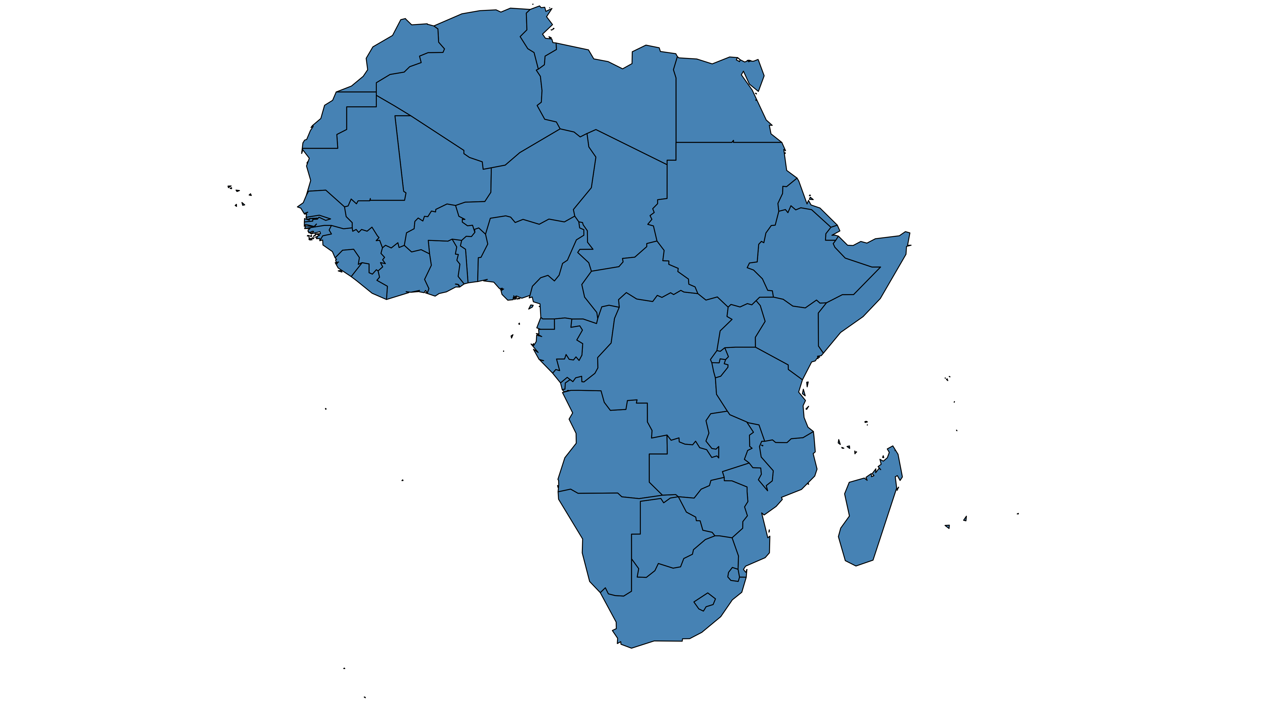
# Keep only data concerning Africa
africa <- my_sf[my_sf$REGION == 2, ]

# Plot africa
par(mar = c(0, 0, 0, 0))
plot(st_geometry(africa),
  xlim = c(-20, 60), ylim = c(-40, 35),
  col = "steelblue", lwd = 0.5
)
Simplify the geospatial object
It’s a common task to simplify the geospatial object. Basically, it decreases the border precision which results in a lighter object that will be plotted faster.
The rmapshaper package offers the
ms_simplify() function to makes the simplification. Play
with the keep argument to control simplification rate.

# Simplification with rmapshaper
library("rmapshaper")
africaSimple <- ms_simplify(africa, keep = 0.01, keep_shapes = TRUE)

# Plot it
par(mar = c(0, 0, 0, 0))
plot(st_geometry(africaSimple),
  xlim = c(-20, 60), ylim = c(-40, 35),
  col = "#59b2a3", lwd = 0.5
)
Compute region centroid
Another common task is to compute the centroid of each region to add
labels. This is doable using the st_centroid() function of
the sf package.
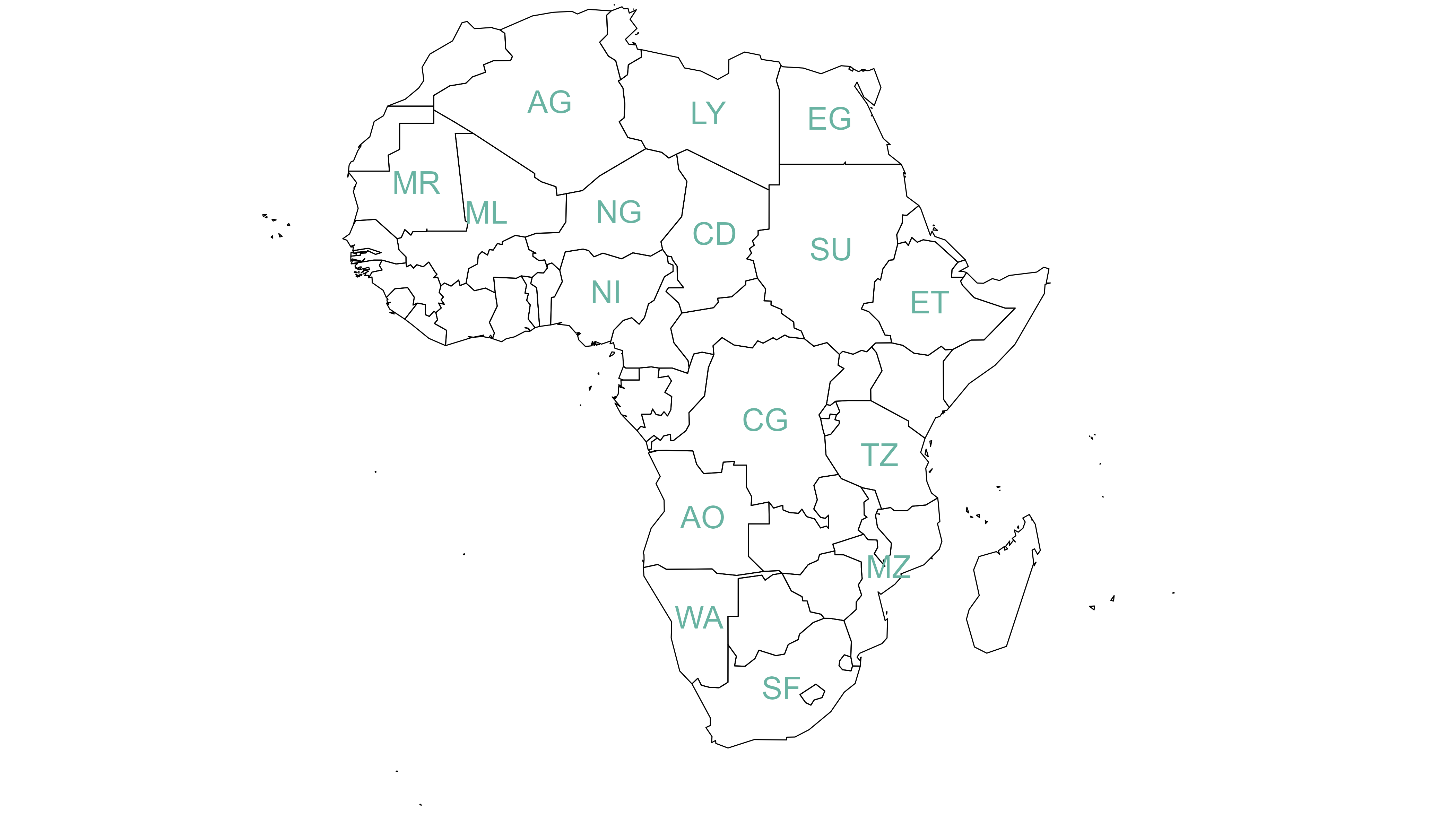
# The st_centroid function computes the centroid of each region:
# st_centroid(africa, of_largest_polygon = TRUE)

# select big countries only
africaBig <- africa[which(africa$AREA > 75000), ]

centroids <- st_centroid(africaBig, of_largest_polygon = TRUE)
# Small manipulation to add coordinates as columns
centers <- cbind(centroids, st_coordinates(centroids))

# Show it on the map
par(mar = c(0, 0, 0, 0))
plot(st_geometry(africa), xlim = c(-20, 60), ylim = c(-40, 35), lwd = 0.5)
text(centers$X, centers$Y, centers$FIPS, cex = .9, col = "#69b3a2")