CatastRo provide access to different API services of the Spanish Cadastre. With CatastRo it is possible to download official information of addresses, properties, parcels and buildings.
OVCCoordenadas Service
The OVCCoordenadas
service allows to retrieve the coordinates of a known cadastral
reference (geocoding). It is also possible to retrieve the cadastral
references around a specific pair of coordinates (reverse geocoding).
CatastRo returns the results on a tibble
format. This functionality is described in detail in the corresponding
vignette (see
vignette("ovcservice", package = "CatastRo")).
INSPIRE Services
The INSPIRE Directive aims to create a European Union spatial data infrastructure for the purposes of EU environmental policies and policies or activities which may have an impact on the environment. This European Spatial Data Infrastructure will enable the sharing of environmental spatial information among public sector organisations, facilitate public access to spatial information across Europe and assist in policy-making across boundaries.
From https://knowledge-base.inspire.ec.europa.eu/overview_en
The implementation of the INSPIRE directive on the Spanish Cadastre (see Catastro INSPIRE) allows to retrieve spatial objects from the database of the cadastre:
-
Vector objects: Parcels, addresses, buildings,
cadastral zones and more. These objects are provided by
CatastRo as
sfobjects as provided by the sf package. -
Imagery: Image layers representing the same
information than the vector objects. These objects are provided by
CatastRo as
SpatRasterobjects as provided by the terra package.
Note that the coverage of this service is 95% of the Spanish territory, excluding Basque Country and Navarre1 that have their own independent cadastral offices.
There are three types of functions, each one querying a different service:
ATOM service: The ATOM service allows to batch-download vector objects of different cadastral elements for a specific municipality.
WFS service: The WFS service allows to download vector objects of specific cadastral elements. Note that there are some restrictions on the extension and number of elements to query. For batch-downloading the ATOM service is preferred.
WMS service: This service allows to download georeferenced images of different cadastral elements.
Examples
Working with layers
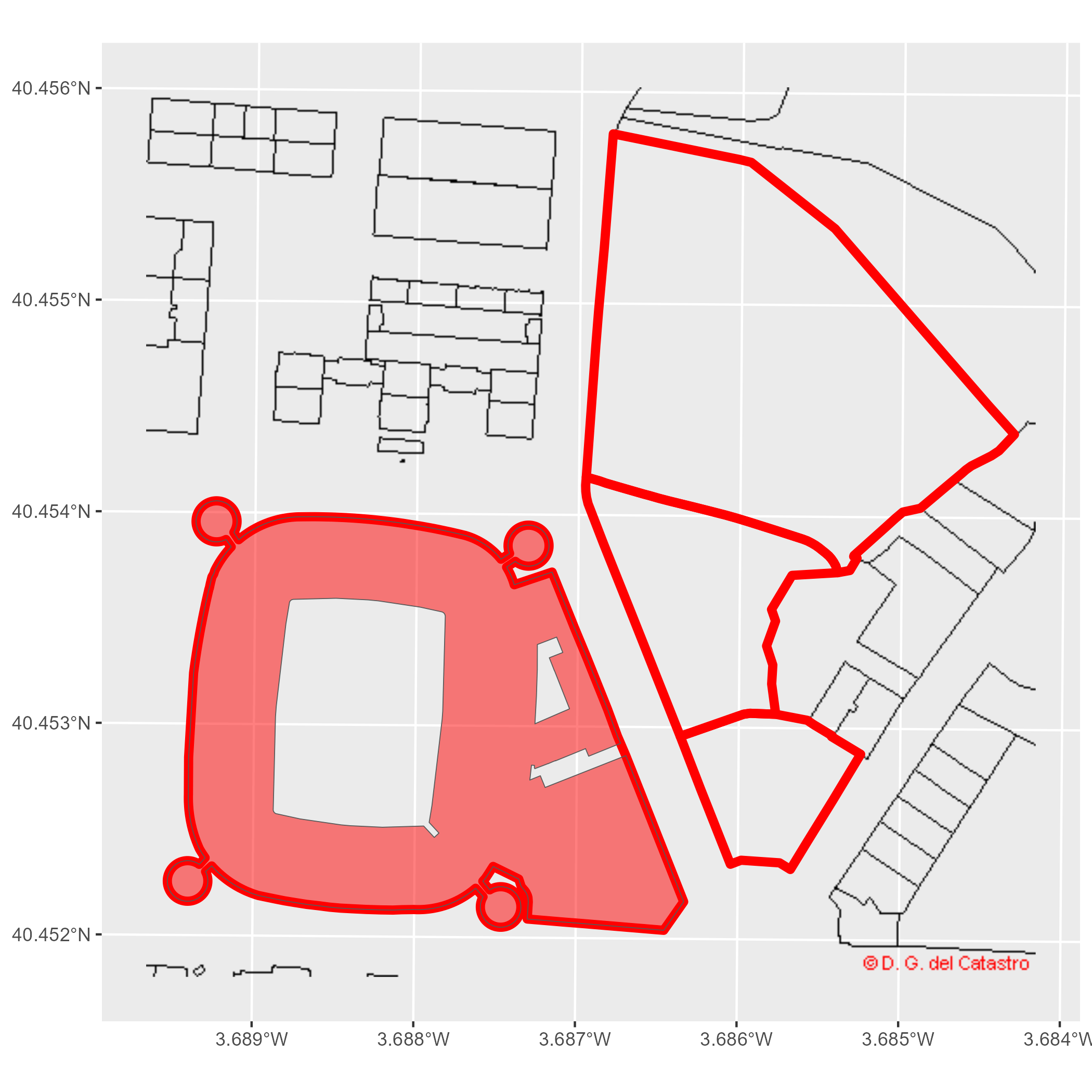
On this example we would demonstrate some of the main capabilities of the package by recreating a cadastral map of the surroundings of the Santiago Bernabéu Stadium. We would make use of the WMS and WFS services to get different layers in order to show some of the capabilities of the package:
# Extract building by bounding box
# Check https://boundingbox.klokantech.com/

library(CatastRo)

stadium <- catr_wfs_get_buildings_bbox(
  c(-3.6891446916, 40.4523311971, -3.687462138, 40.4538643165),
  srs = 4326
)

# Now extract cadastral parcels. We can use spatial objects on the query

stadium_parcel <- catr_wfs_get_parcels_bbox(stadium)

# Project for tiles

stadium_parcel_pr <- sf::st_transform(stadium_parcel, 25830)

# Extract imagery: Labels of the parcel

labs <- catr_wms_get_layer(stadium_parcel_pr,
  what = "parcel",
  styles = "BoundariesOnly",
  srs = 25830
)

# Plot
library(ggplot2)
library(tidyterra) # For terra tiles

ggplot() +
  geom_spatraster_rgb(data = labs) +
  geom_sf(data = stadium_parcel_pr, fill = NA, col = "red", linewidth = 2) +
  geom_sf(data = stadium, fill = "red", alpha = .5) +
  coord_sf(crs = 25830)
Example: Santiago Bernabeu
Thematic maps
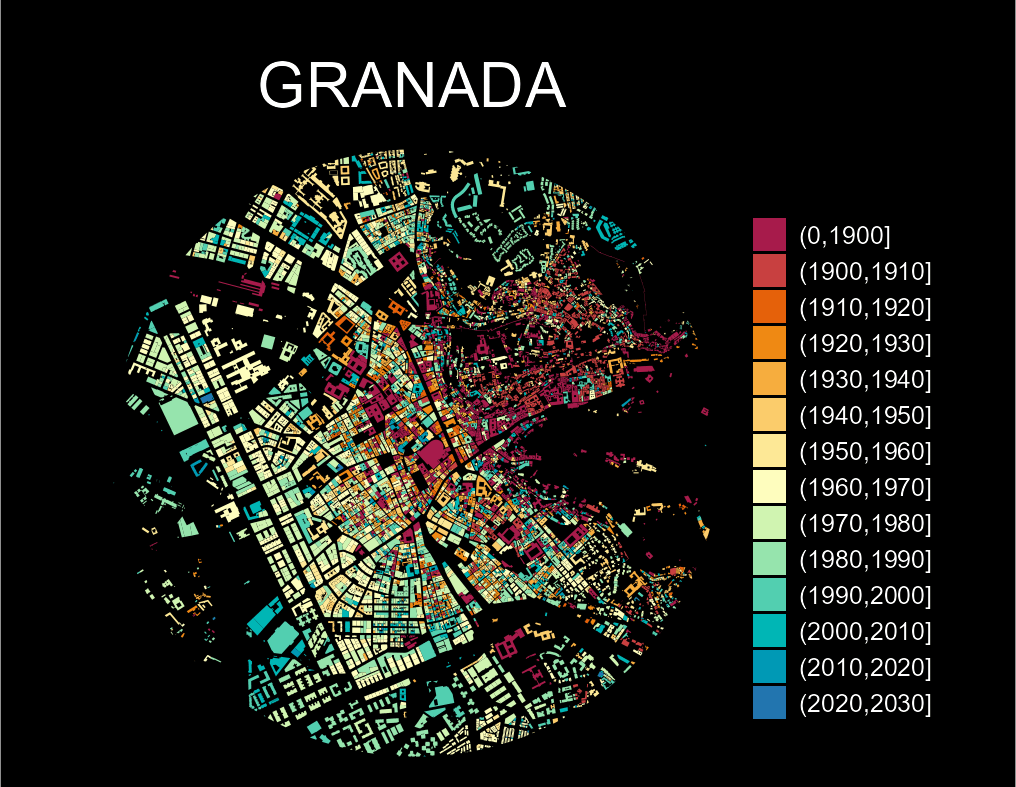
We can create also thematic maps using the information available on the spatial objects. We would produce a visualization of the urban growth of Granada using CatastRo, replicating the map produced by Dominic Royé on his post Visualize urban growth, using the ATOM services.
In first place, we extract the coordinates of the city center of Granada using mapSpain:
library(dplyr)
library(sf)
library(mapSpain)

# Use mapSpain for getting the coords

city <- esp_get_capimun(munic = "^Granada$")
Next step consists on extracting the buildings using the ATOM
service. We would use also the function
catr_get_code_from_coords() to identify the code of Granada
in the Cadastre, and we would download the buildings with
catr_atom_get_buildings().
city_catr_code <- catr_get_code_from_coords(city)

city_catr_code
#> # A tibble: 1 × 12
#>   munic  catr_to catr_munic catrcode cpro  cmun  inecode nm    cd    cmc   cp
#>   <chr>  <chr>   <chr>      <chr>    <chr> <chr> <chr>   <chr> <chr> <chr> <chr>
#> 1 GRANA… 18      900        18900    18    087   18087   GRAN… 18    900   18
#> # ℹ 1 more variable: cm <chr>

city_bu <- catr_atom_get_buildings(city_catr_code$catrcode)
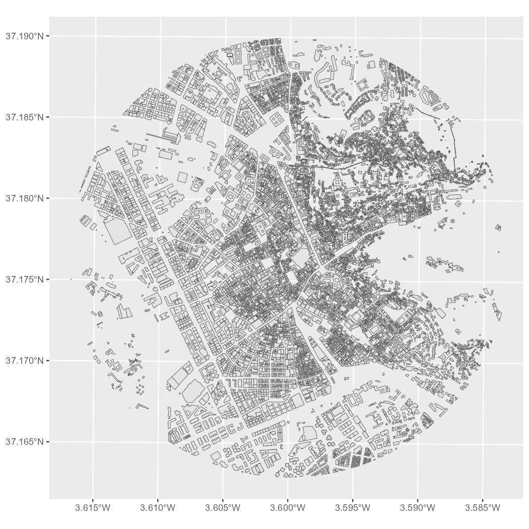
Next step for creating the visualization is to limit the analysis to a circle of radius 1.5 km around the city center:
buff <- city %>%
  # Adjust CRS to 25830: (Buildings)
  st_transform(st_crs(city_bu)) %>%
  # Buffer
  st_buffer(1500)


# Cut buildings

dataviz <- st_intersection(city_bu, buff)

ggplot(dataviz) +
  geom_sf()
Minimal cadastral map of Granada
Let’s extract now the construction year, available in the column
beginning:
# Extract 4 initial positions
year <- substr(dataviz$beginning, 1, 4)

# Replace all that doesn't look as a number with 0000
year[!(year %in% 0:2500)] <- "0000"


# To numeric
year <- as.integer(year)

# New column
dataviz <- dataviz %>%
  mutate(year = year)
Last step is to create groups based on the year and create the data
visualization. We use here the function cut() to create
classes for every decade starting in year 1900:
dataviz <- dataviz %>%
  mutate(year_cat = cut(year,
    breaks = c(0, seq(1900, 2030, by = 10)),
    dig.lab = 4
  ))


ggplot(dataviz) +
  geom_sf(aes(fill = year_cat), color = NA, na.rm = TRUE) +
  scale_fill_manual(
    values = hcl.colors(15, "Spectral"),
    na.translate = FALSE
  ) +
  theme_void() +
  labs(title = "GRANADA", fill = "") +
  theme(
    panel.background = element_rect(fill = "black"),
    plot.background = element_rect(fill = "black"),
    legend.justification = .5,
    legend.text = element_text(
      colour = "white",
      size = 12
    ),
    plot.title = element_text(
      colour = "white", hjust = .5,
      margin = margin(t = 30),
      size = 30
    ),
    plot.caption = element_text(
      colour = "white",
      margin = margin(b = 20), hjust = .5
    ),
    plot.margin = margin(r = 40, l = 40)
  )
Granada: Urban growth
References
- Royé D (2019). “Visualize urban growth.” https://dominicroye.github.io/en/2019/visualize-urban-growth/.
