Visualise SpatRaster objects as images — geom_spatraster

This geom is used to visualise SpatRaster objects (see terra::rast()) as RGB images. The layers are combined such that they represent the red, green and blue channel.

For plotting SpatRaster objects by layer values use geom_spatraster().

The underlying implementation is based on ggplot2::geom_raster().

Usage

geom_spatraster_rgb(
  mapping = aes(),
  data,
  interpolate = TRUE,
  r = 1,
  g = 2,
  b = 3,
  alpha = 1,
  maxcell = 5e+05,
  max_col_value = 255,
  ...
)

Source

Based on the layer_spatial() implementation on ggspatial package. Thanks to Dewey Dunnington and ggspatial contributors.

Arguments

mapping

Ignored.

data

A SpatRaster object.

interpolate

If TRUE interpolate linearly, if FALSE (the default) don't interpolate.

r, g, b

Integer representing the number of layer of data to be considered as the red (r), green (g) and blue (b) channel.

alpha

The alpha transparency, a number in [0,1], see argument alpha in hsv.

maxcell

positive integer. Maximum number of cells to use for the plot.

max_col_value

Number giving the maximum of the color values range. When this is 255 (the default), the result is computed most efficiently. See grDevices::rgb().

...

Other arguments passed on to layer()'s params argument. These arguments broadly fall into one of 4 categories below. Notably, further arguments to the position argument, or aesthetics that are required can not be passed through .... Unknown arguments that are not part of the 4 categories below are ignored.

Static aesthetics that are not mapped to a scale, but are at a fixed value and apply to the layer as a whole. For example, colour = "red" or linewidth = 3. The geom's documentation has an Aesthetics section that lists the available options. The 'required' aesthetics cannot be passed on to the params. Please note that while passing unmapped aesthetics as vectors is technically possible, the order and required length is not guaranteed to be parallel to the input data.
When constructing a layer using a stat_*() function, the ... argument can be used to pass on parameters to the geom part of the layer. An example of this is stat_density(geom = "area", outline.type = "both"). The geom's documentation lists which parameters it can accept.
Inversely, when constructing a layer using a geom_*() function, the ... argument can be used to pass on parameters to the stat part of the layer. An example of this is geom_area(stat = "density", adjust = 0.5). The stat's documentation lists which parameters it can accept.
The key_glyph argument of layer() may also be passed on through .... This can be one of the functions described as key glyphs, to change the display of the layer in the legend.

Value

A ggplot2 layer

terra equivalent

terra::plotRGB()

Aesthetics

No aes() is required. In fact, aes() will be ignored.

Coords

When the SpatRaster does not present a crs (i.e., terra::crs(rast) == "") the geom does not make any assumption on the scales.

On SpatRaster that have a crs, the geom uses ggplot2::coord_sf() to adjust the scales. That means that also the SpatRaster may be reprojected.

Examples

# \donttest{

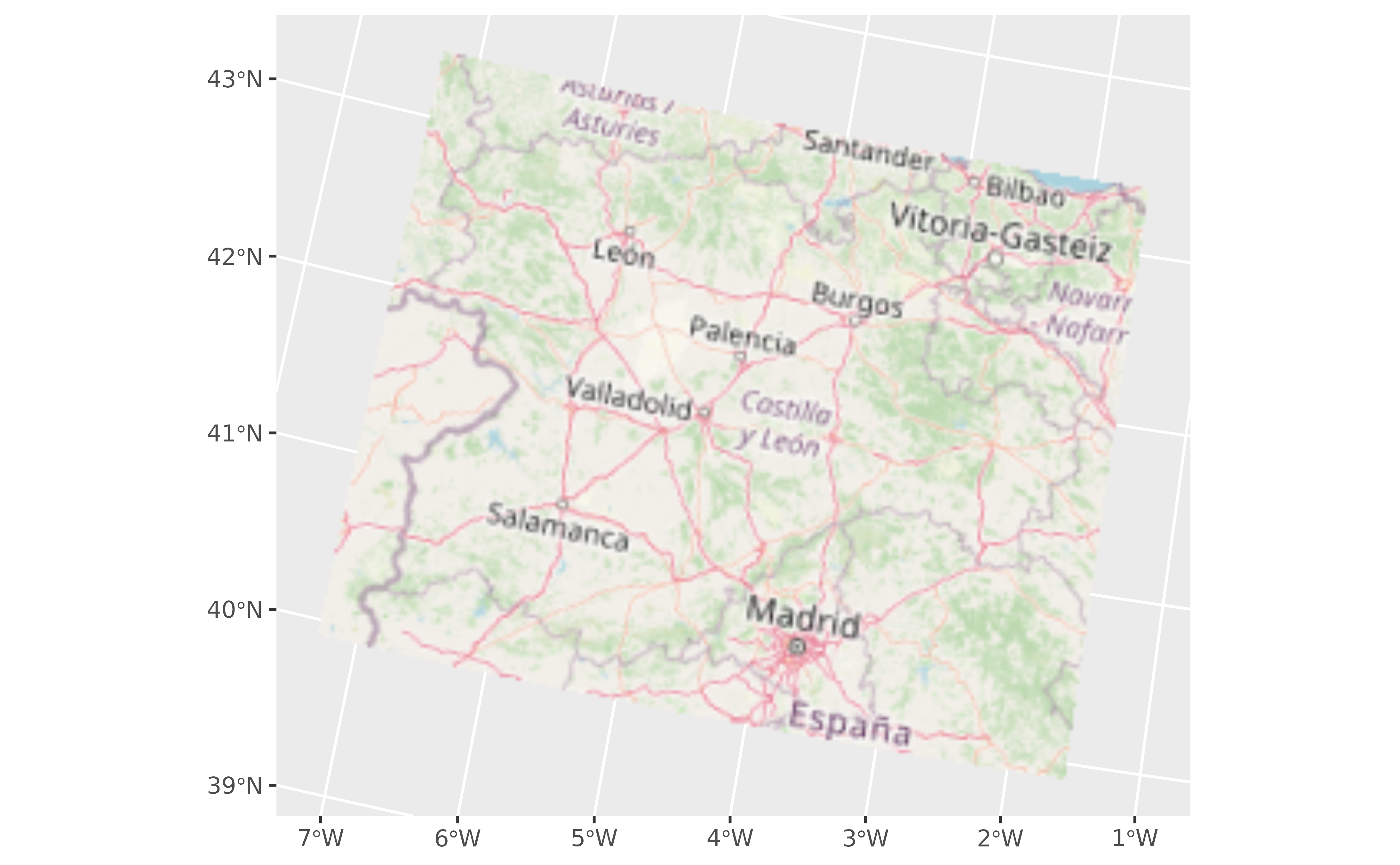
# Tile of Castille and Leon (Spain) from OpenStreetMap
file_path <- system.file("extdata/cyl_tile.tif", package = "tidyterra")

library(terra)
tile <- rast(file_path)

library(ggplot2)


ggplot() +
  geom_spatraster_rgb(data = tile) +
  # You can use coord_sf
  coord_sf(crs = 3035)


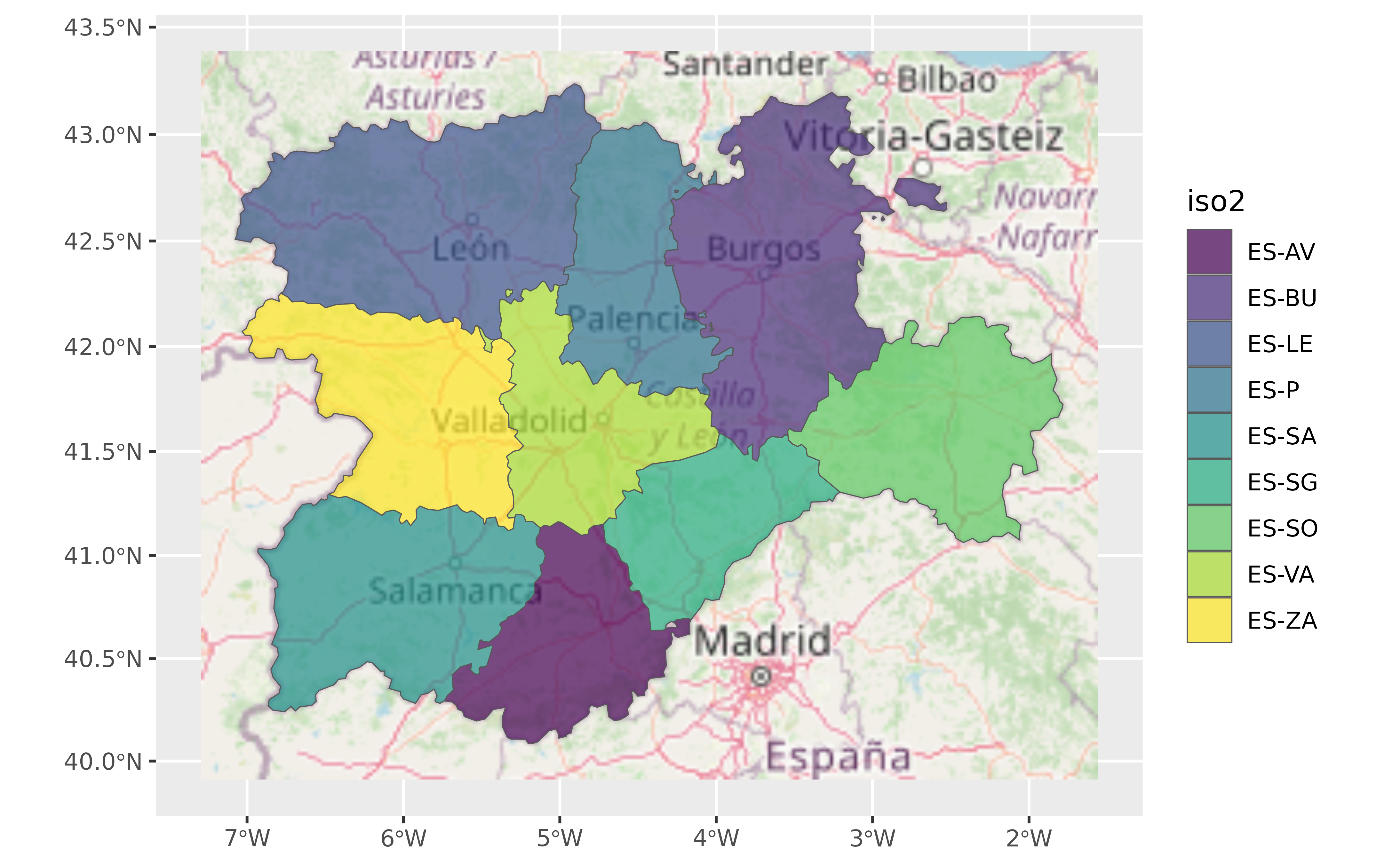
# Combine with sf objects
vect_path <- system.file("extdata/cyl.gpkg", package = "tidyterra")

cyl_sf <- sf::st_read(vect_path)
#> Reading layer `cyl' from data source 
#>   `D:\a\_temp\Library\tidyterra\extdata\cyl.gpkg' using driver `GPKG'
#> Simple feature collection with 9 features and 3 fields
#> Geometry type: MULTIPOLYGON
#> Dimension:     XY
#> Bounding box:  xmin: 2892687 ymin: 2017622 xmax: 3341372 ymax: 2361600
#> Projected CRS: ETRS89-extended / LAEA Europe

ggplot(cyl_sf) +
  geom_spatraster_rgb(data = tile) +
  geom_sf(aes(fill = iso2)) +
  coord_sf(crs = 3857) +
  scale_fill_viridis_d(alpha = 0.7)

# }

Visualise `SpatRaster` objects as images