Visualise SpatRaster objects — geom_spatraster • tidyterra

This geom is used to visualise SpatRaster objects (see terra::rast()). The geom is designed for visualise the object by layers, as terra::plot() does.

For plotting SpatRaster objects as map tiles (i.e. RGB SpatRaster), use geom_spatraster_rgb().

The underlying implementation is based on ggplot2::geom_raster().

stat_spatraster() complements geom_spatraster() when you need to change the geom.

Usage

geom_spatraster(
  mapping = aes(),
  data,
  na.rm = TRUE,
  show.legend = NA,
  inherit.aes = FALSE,
  interpolate = FALSE,
  maxcell = 5e+05,
  use_coltab = TRUE,
  mask_projection = FALSE,
  ...
)

stat_spatraster(
  mapping = aes(),
  data,
  geom = "raster",
  na.rm = TRUE,
  show.legend = NA,
  inherit.aes = FALSE,
  maxcell = 5e+05,
  ...
)

Source

Based on the layer_spatial() implementation on ggspatial package. Thanks to Dewey Dunnington and ggspatial contributors.

Arguments

mapping

Set of aesthetic mappings created by ggplot2::aes(). See Aesthetics specially in the use of fill aesthetic.

data

A SpatRaster object.

na.rm

If TRUE, the default, missing values are silently removed. If FALSE, missing values are removed with a warning.

show.legend

logical. Should this layer be included in the legends? NA, the default, includes if any aesthetics are mapped. FALSE never includes, and TRUE always includes. It can also be a named logical vector to finely select the aesthetics to display. To include legend keys for all levels, even when no data exists, use TRUE. If NA, all levels are shown in legend, but unobserved levels are omitted.

inherit.aes

If FALSE, overrides the default aesthetics, rather than combining with them.

interpolate

If TRUE interpolate linearly, if FALSE (the default) don't interpolate.

maxcell

Positive integer. Maximum number of cells to use for the plot.

use_coltab

Logical. Only applicable to SpatRaster objects that have an associated coltab. Should the coltab be used on the plot? See also scale_fill_coltab().

mask_projection

Logical, defaults to FALSE. If TRUE, mask out areas outside the input extent. For example, to avoid data wrapping around the date-line in Equal Area projections. This argument is passed to terra::project() when reprojecting the SpatRaster.

...

Other arguments passed on to layer()'s params argument. These arguments broadly fall into one of 4 categories below. Notably, further arguments to the position argument, or aesthetics that are required can not be passed through .... Unknown arguments that are not part of the 4 categories below are ignored.

Static aesthetics that are not mapped to a scale, but are at a fixed value and apply to the layer as a whole. For example, colour = "red" or linewidth = 3. The geom's documentation has an Aesthetics section that lists the available options. The 'required' aesthetics cannot be passed on to the params. Please note that while passing unmapped aesthetics as vectors is technically possible, the order and required length is not guaranteed to be parallel to the input data.
When constructing a layer using a stat_*() function, the ... argument can be used to pass on parameters to the geom part of the layer. An example of this is stat_density(geom = "area", outline.type = "both"). The geom's documentation lists which parameters it can accept.
Inversely, when constructing a layer using a geom_*() function, the ... argument can be used to pass on parameters to the stat part of the layer. An example of this is geom_area(stat = "density", adjust = 0.5). The stat's documentation lists which parameters it can accept.
The key_glyph argument of layer() may also be passed on through .... This can be one of the functions described as key glyphs, to change the display of the layer in the legend.

geom

Geom used to display the data. Recommended values for SpatRaster are "raster" (the default), "point", "text" and "label".

Value

A ggplot2 layer

terra equivalent

terra::plot()

Coords

When the SpatRaster does not present a CRS (i.e., terra::crs(rast) == "") the geom does not make any assumption on the scales.

On SpatRaster that have a CRS, the geom uses ggplot2::coord_sf() to adjust the scales. That means that also the SpatRaster may be reprojected.

Aesthetics

geom_spatraster() understands the following aesthetics:

fill
alpha

If fill is not provided, geom_spatraster() creates a ggplot2 layer with all the layers of the SpatRaster object. Use facet_wrap(~lyr) to properly display the SpatRaster layers.

If fill is used, it should contain the name of one layer that is present on the SpatRaster (i.e. geom_spatraster(data = rast, aes(fill = <name_of_lyr>)). Names of the layers can be retrieved using names(rast).

Using geom_spatraster(..., mapping = aes(fill = NULL)) or geom_spatraster(..., fill = <color value(s)>) would create a layer with no mapped fill aesthetic.

fill can use computed variables.

For alpha use computed variable. See section Computed variables.

`stat_spatraster()`

stat_spatraster() understands the same aesthetics as geom_spatraster() when geom = "raster" (the default):

fill
alpha

When geom = "raster", the fill argument behaves as in geom_spatraster(). If another geom is used, stat_spatraster() understands the aesthetics required by that geom, so aes(fill = <name_of_lyr>) is not applicable.

The x and y aesthetics are mapped by default, so you do not need to add them in aes(). In every case, aesthetics should be mapped with computed variables. See Computed variables and Examples.

You can use facet_wrap(~lyr) for creating a faceted plot by each layer of the SpatRaster object. See ggplot2::facet_wrap() for details.

Computed variables

This geom computes internally some variables that are available for use as aesthetics, using (for example) aes(alpha = after_stat(value)) (see ggplot2::after_stat()).

after_stat(value): Values of the SpatRaster.
after_stat(lyr): Name of the layer.

Examples

# \donttest{
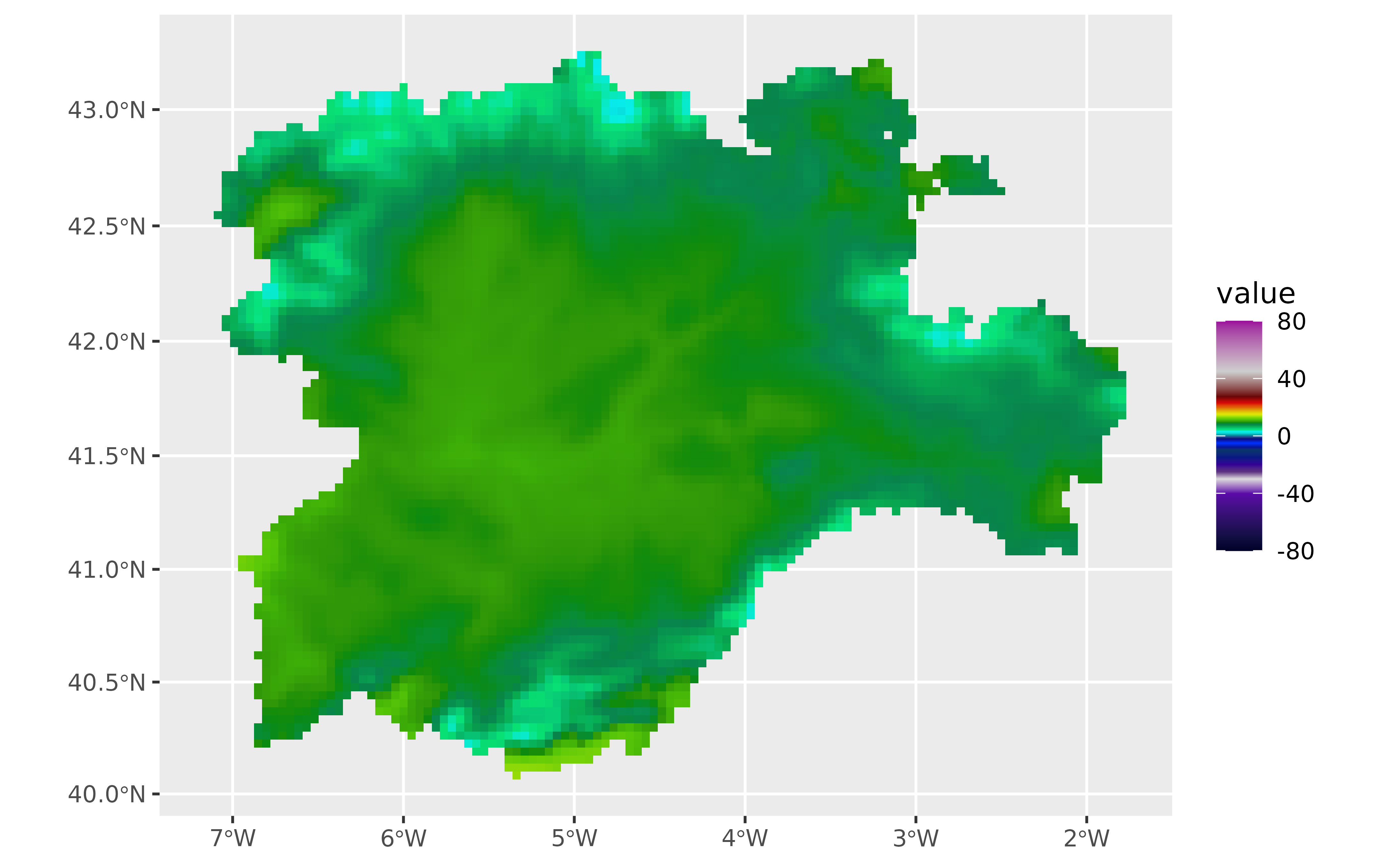
# Avg temperature on spring in Castile and Leon (Spain)
file_path <- system.file("extdata/cyl_temp.tif", package = "tidyterra")

library(terra)
temp_rast <- rast(file_path)

library(ggplot2)

# Display a single layer
names(temp_rast)
#> [1] "tavg_04" "tavg_05" "tavg_06"

ggplot() +
  geom_spatraster(data = temp_rast, aes(fill = tavg_04)) +
  # You can use coord_sf
  coord_sf(crs = 3857) +
  scale_fill_grass_c(palette = "celsius")


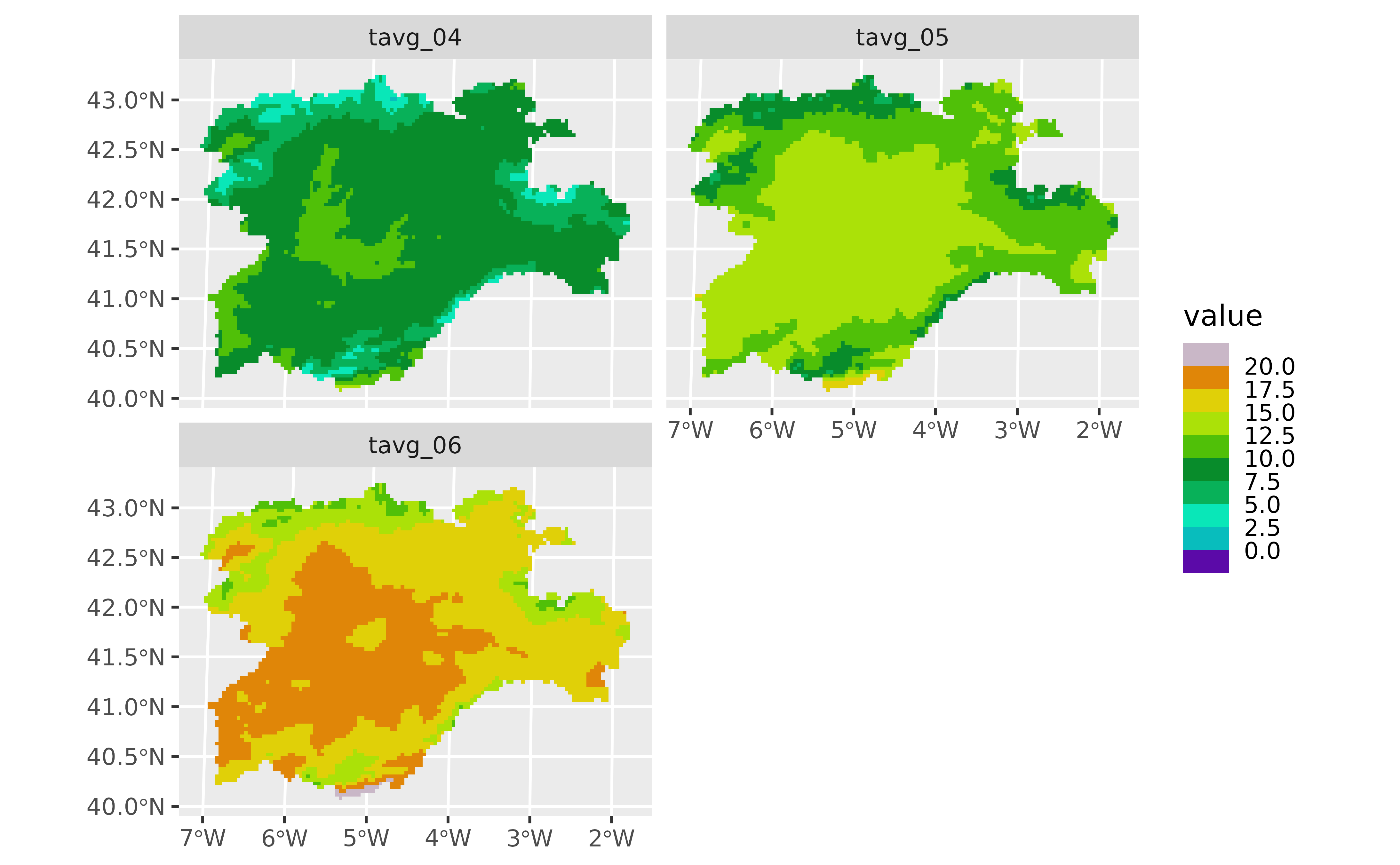
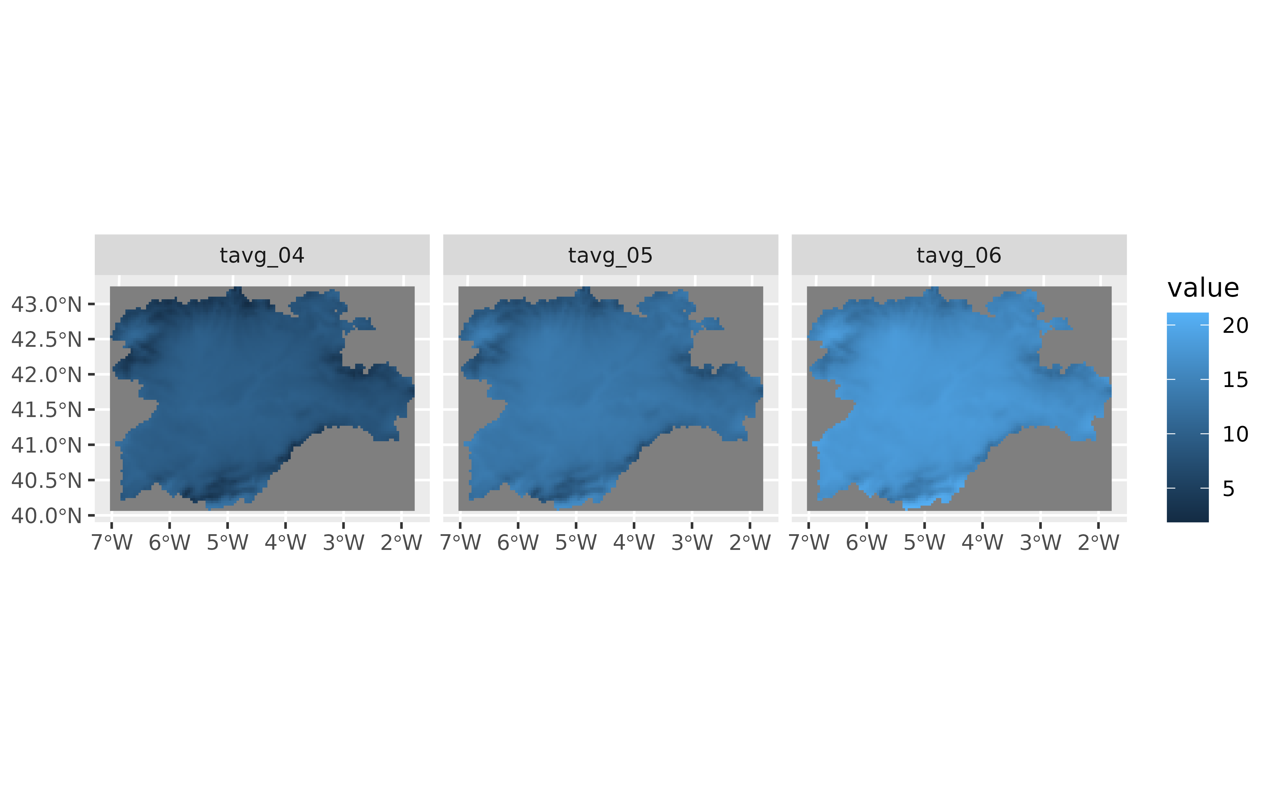
# Display facets
ggplot() +
  geom_spatraster(data = temp_rast) +
  facet_wrap(~lyr, ncol = 2) +
  scale_fill_grass_b(palette = "celsius", breaks = seq(0, 20, 2.5))


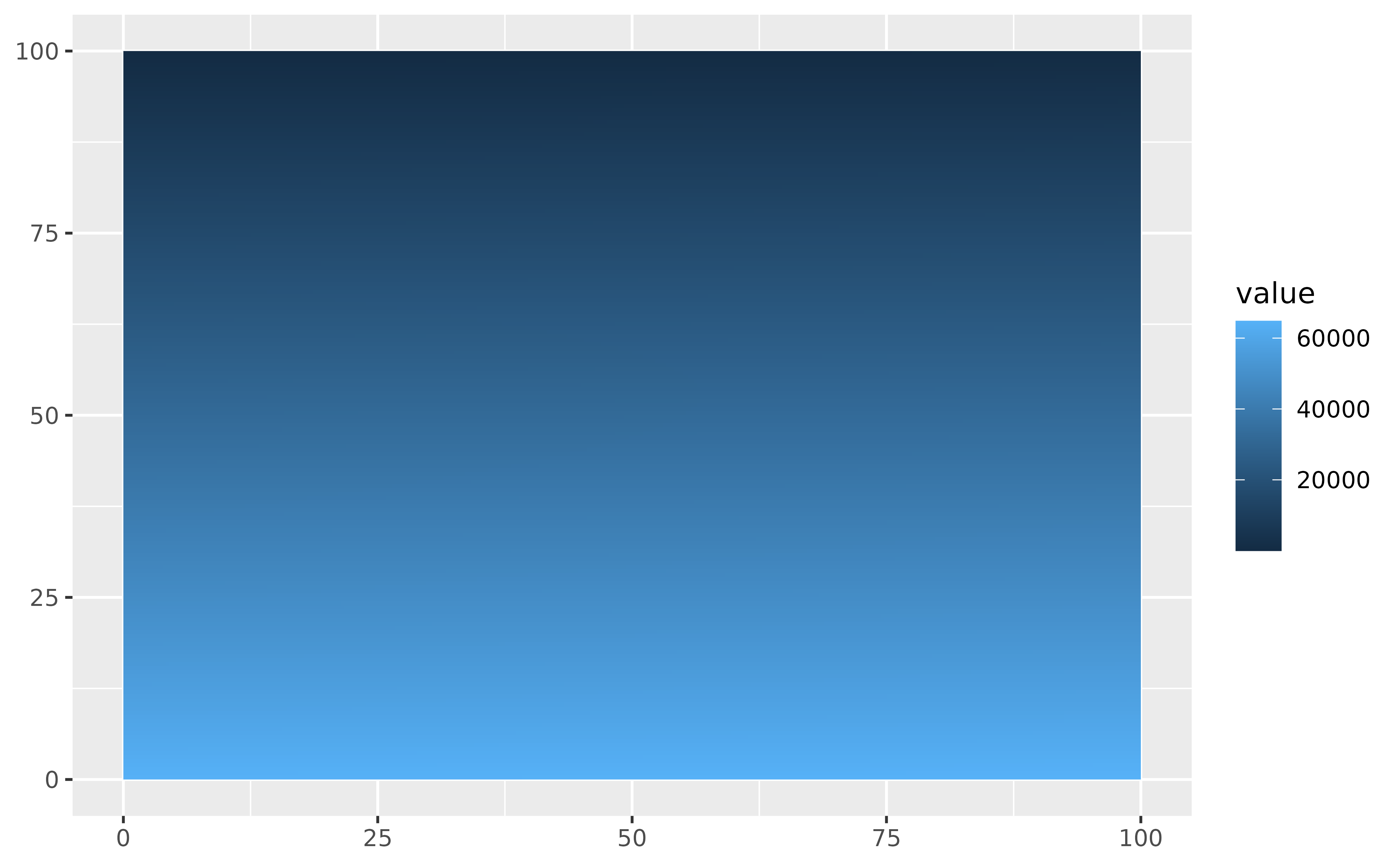
# Non spatial rasters

no_crs <- rast(crs = NA, extent = c(0, 100, 0, 100), nlyr = 1)
values(no_crs) <- seq_len(ncell(no_crs))

ggplot() +
  geom_spatraster(data = no_crs)


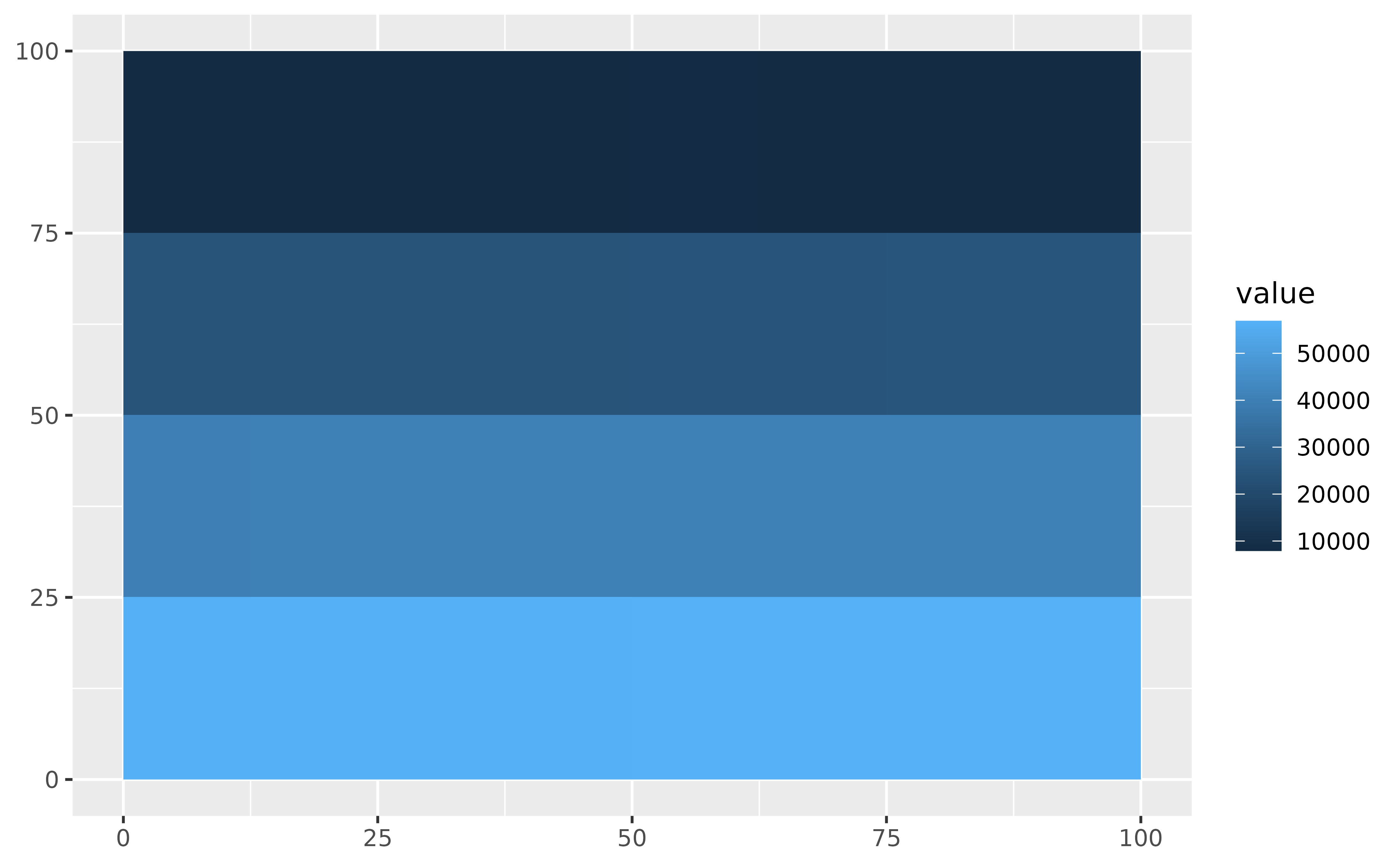
# Downsample

ggplot() +
  geom_spatraster(data = no_crs, maxcell = 25)
#> <SpatRaster> resampled to 32 cells.

# }

# \donttest{
# Using stat_spatraster
# Default
ggplot() +
  stat_spatraster(data = temp_rast) +
  facet_wrap(~lyr)


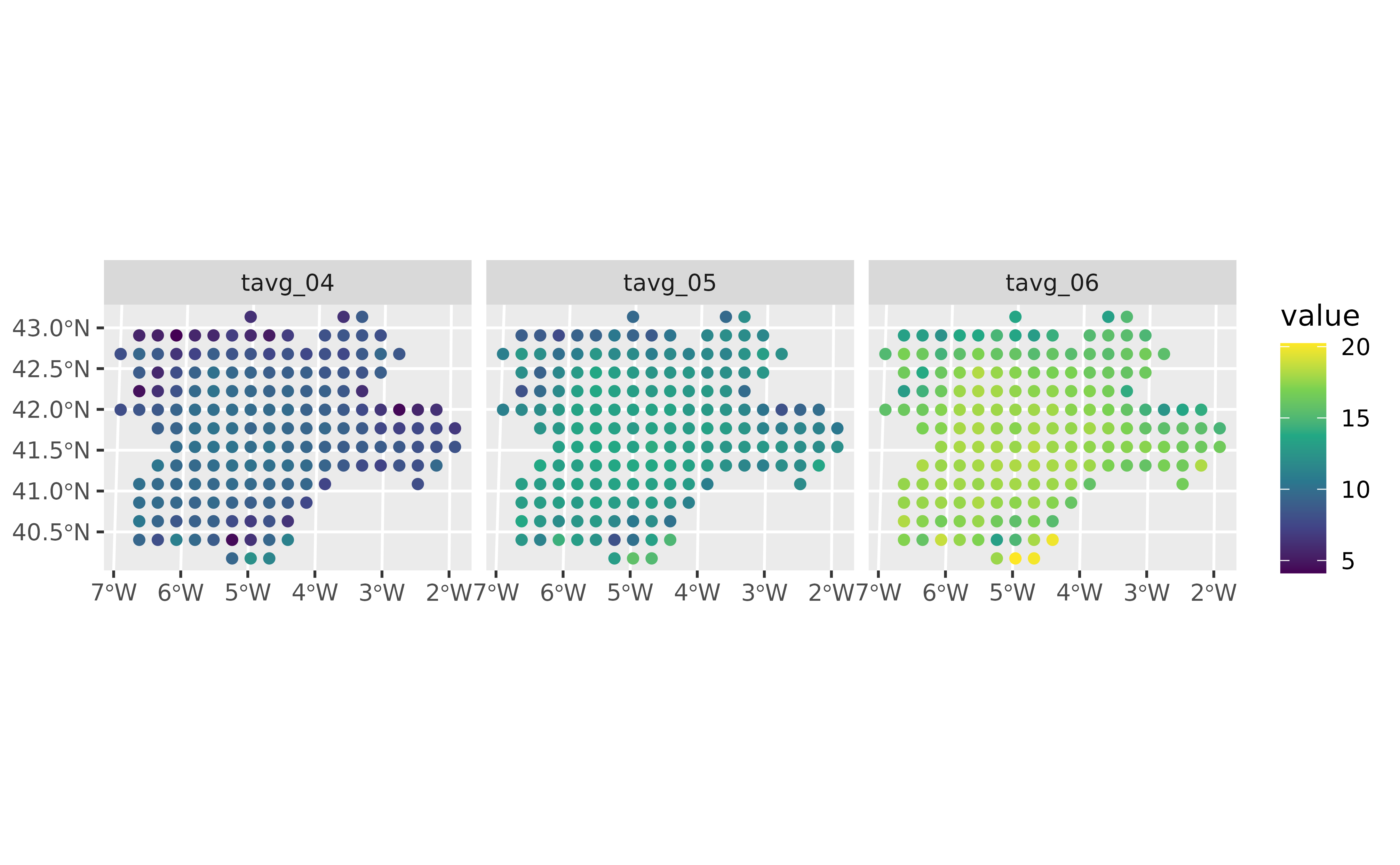
# Using points
ggplot() +
  stat_spatraster(
    data = temp_rast,
    aes(color = after_stat(value)),
    geom = "point", maxcell = 250
  ) +
  scale_colour_viridis_c(na.value = "transparent") +
  facet_wrap(~lyr)
#> <SpatRaster> resampled to 266 cells.


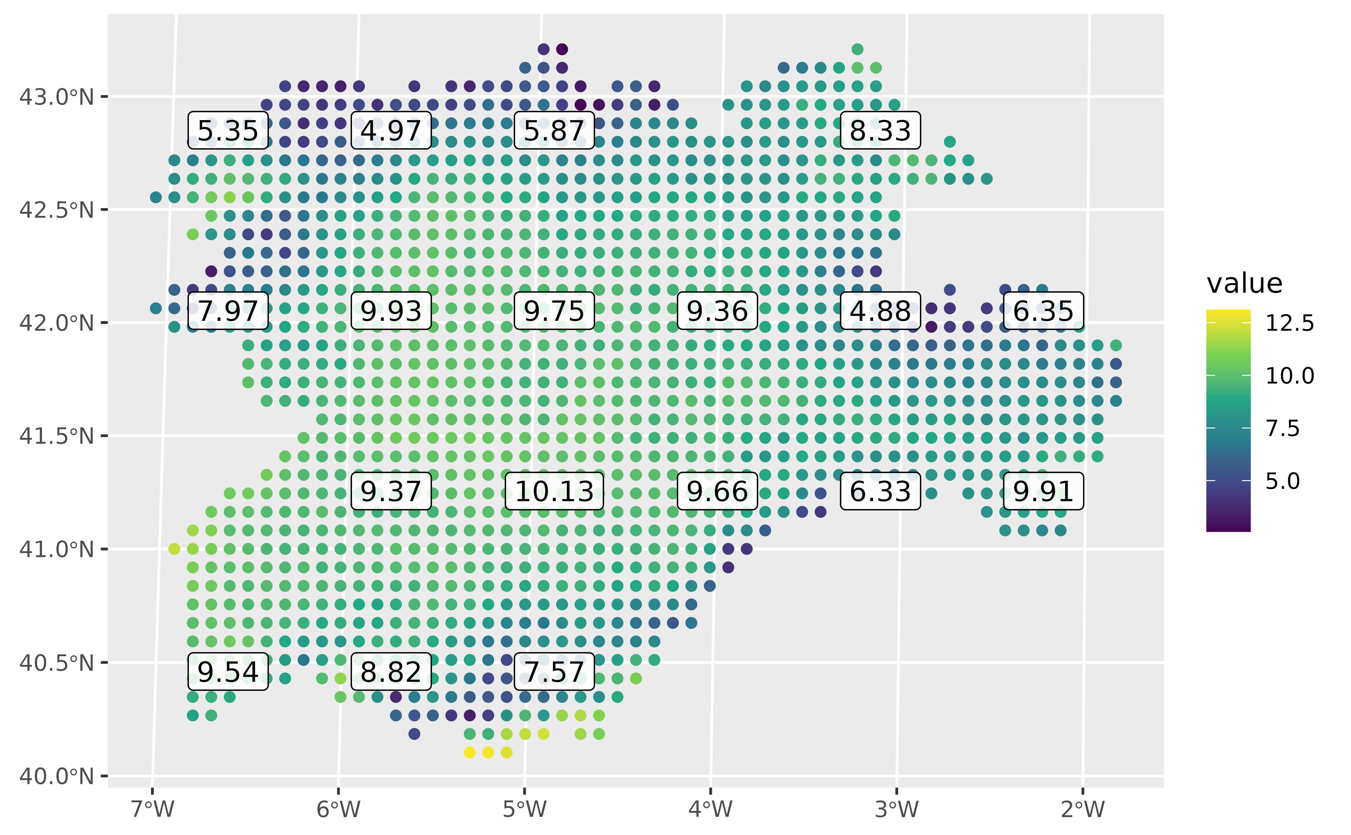
# Using points and labels

r_single <- temp_rast |> select(1)

ggplot() +
  stat_spatraster(
    data = r_single,
    aes(color = after_stat(value)),
    geom = "point",
    maxcell = 2000
  ) +
  stat_spatraster(
    data = r_single,
    aes(label = after_stat(round(value, 2))),
    geom = "label",
    alpha = 0.85,
    maxcell = 20
  ) +
  scale_colour_viridis_c(na.value = "transparent")
#> <SpatRaster> resampled to 2067 cells.
#> <SpatRaster> resampled to 24 cells.

# }

Visualise `SpatRaster` objects