Fortify Spat* objects — fortify.Spat • tidyterra

Fortify SpatRaster and SpatVector objects to data frames. This provides native compatibility with ggplot2::ggplot().

These methods are now implemented as wrappers around tidy.Spat methods.

Usage

# S3 method for class 'SpatRaster'
fortify(
  model,
  data,
  ...,
  .name_repair = c("unique", "check_unique", "universal", "minimal", "unique_quiet",
    "universal_quiet"),
  maxcell = terra::ncell(model) * 1.1,
  pivot = FALSE
)

# S3 method for class 'SpatVector'
fortify(model, data, ...)

# S3 method for class 'SpatGraticule'
fortify(model, data, ...)

# S3 method for class 'SpatExtent'
fortify(model, data, ..., crs = "")

Arguments

model

A SpatRaster created with terra::rast(), a SpatVector created with terra::vect(), a SpatGraticule (see terra::graticule()) or a SpatExtent (see terra::ext()).

data

Not used by this method.

...

Ignored by these methods.

.name_repair

Treatment of problematic column names:

"minimal": No name repair or checks, beyond basic existence,
"unique": Make sure names are unique and not empty,
"check_unique": (default value), no name repair, but check they are unique,
"universal": Make the names unique and syntactic
"unique_quiet": Same as "unique", but "quiet"
"universal_quiet": Same as "universal", but "quiet"
a function: apply custom name repair (e.g., .name_repair = make.names for names in the style of base R).
A purrr-style anonymous function, see rlang::as_function()

This argument is passed on as repair to vctrs::vec_as_names(). See there for more details on these terms and the strategies used to enforce them.

maxcell

Positive integer. Maximum number of cells to use for the plot.

pivot

Logical. When TRUE, a SpatRaster is returned in long format. When FALSE (the default), it is returned as a data frame with one column per layer. See Details.

crs

Input that includes or represents a CRS. It can be an sf or sfc object, a SpatRaster or SpatVector object, a crs object from sf::st_crs(), a character string (for example a PROJ string), or an integer representing an EPSG code.

Value

fortify.SpatVector(), fortify.SpatGraticule() and fortify.SpatExtent() return a sf object.

fortify.SpatRaster() returns a tibble. See Methods.

Methods

Implementation of the generic ggplot2::fortify() methods for Spat* objects.

`SpatRaster`

Returns a tibble that can be used with ggplot2::geom_*, such as ggplot2::geom_point() and ggplot2::geom_raster().

The resulting tibble includes coordinates in the x and y columns. The values of each layer are added as extra columns using the layer names from the SpatRaster.

The CRS of the SpatRaster can be retrieved with attr(fortifiedSpatRaster, "crs").

You can convert the fortified object back to a SpatRaster with as_spatraster().

When pivot = TRUE, the SpatRaster is fortified in long format (see tidyr::pivot_longer()). The fortified object has the following columns:

x, y: Coordinates of the cell center in the corresponding CRS.
lyr: Name of the SpatRaster layer associated with value.
value: Cell value for the corresponding lyr.

This option can be useful when combining several geom_* layers or when faceting.

`SpatVector`, `SpatGraticule` and `SpatExtent`

Returns an sf object that can be used with ggplot2::geom_sf().

Examples

# \donttest{

# Demonstrate use with ggplot2.
library(ggplot2)

# Get a SpatRaster.
r <- system.file("extdata/volcano2.tif", package = "tidyterra") |>
  terra::rast() |>
  terra::project("EPSG:4326")

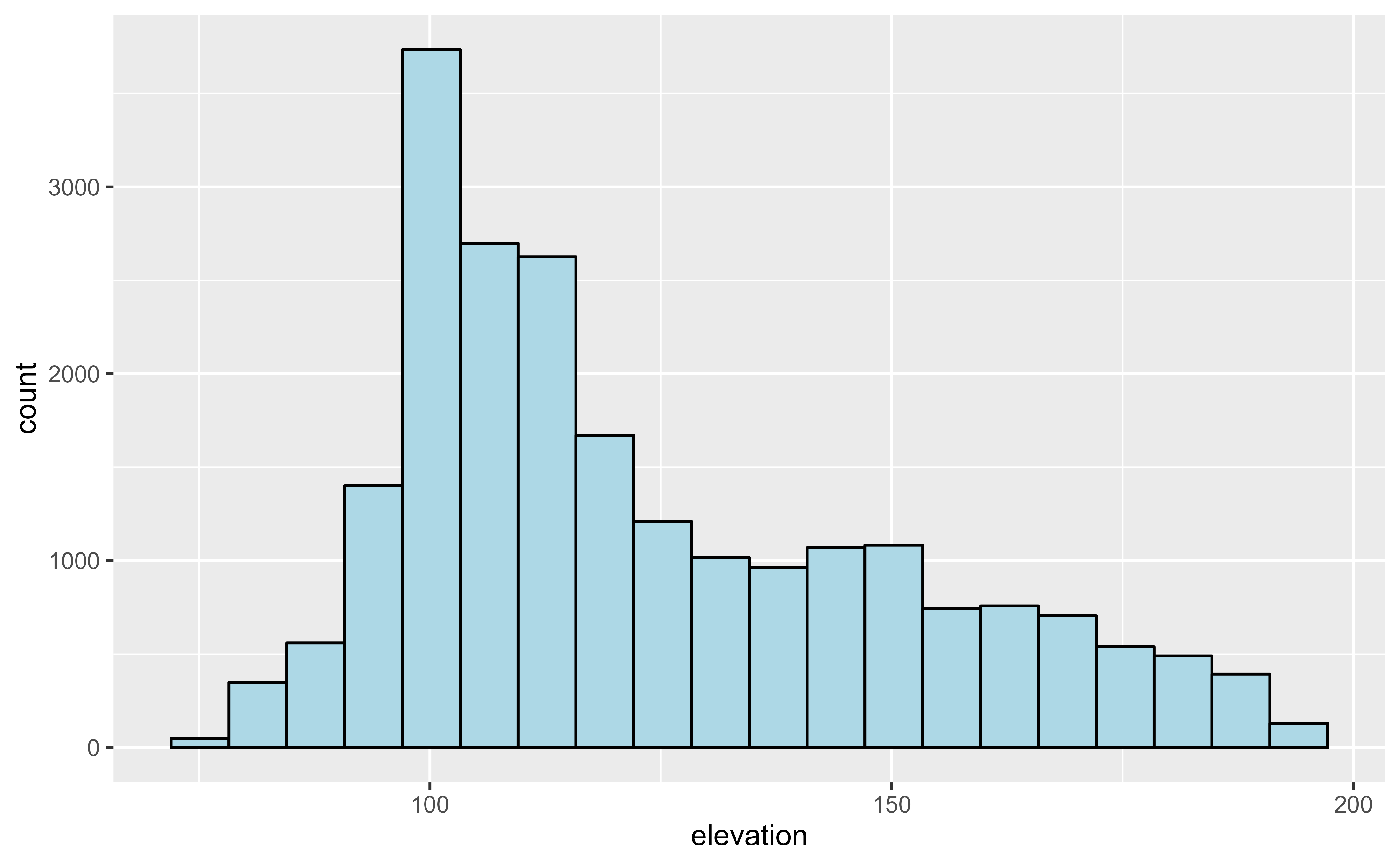
# You can now use a SpatRaster with any geom.
ggplot(r, maxcell = 50) +
  geom_histogram(aes(x = elevation),
    bins = 20, fill = "lightblue",
    color = "black"
  )
#> <SpatRaster> resampled to 56 cells.


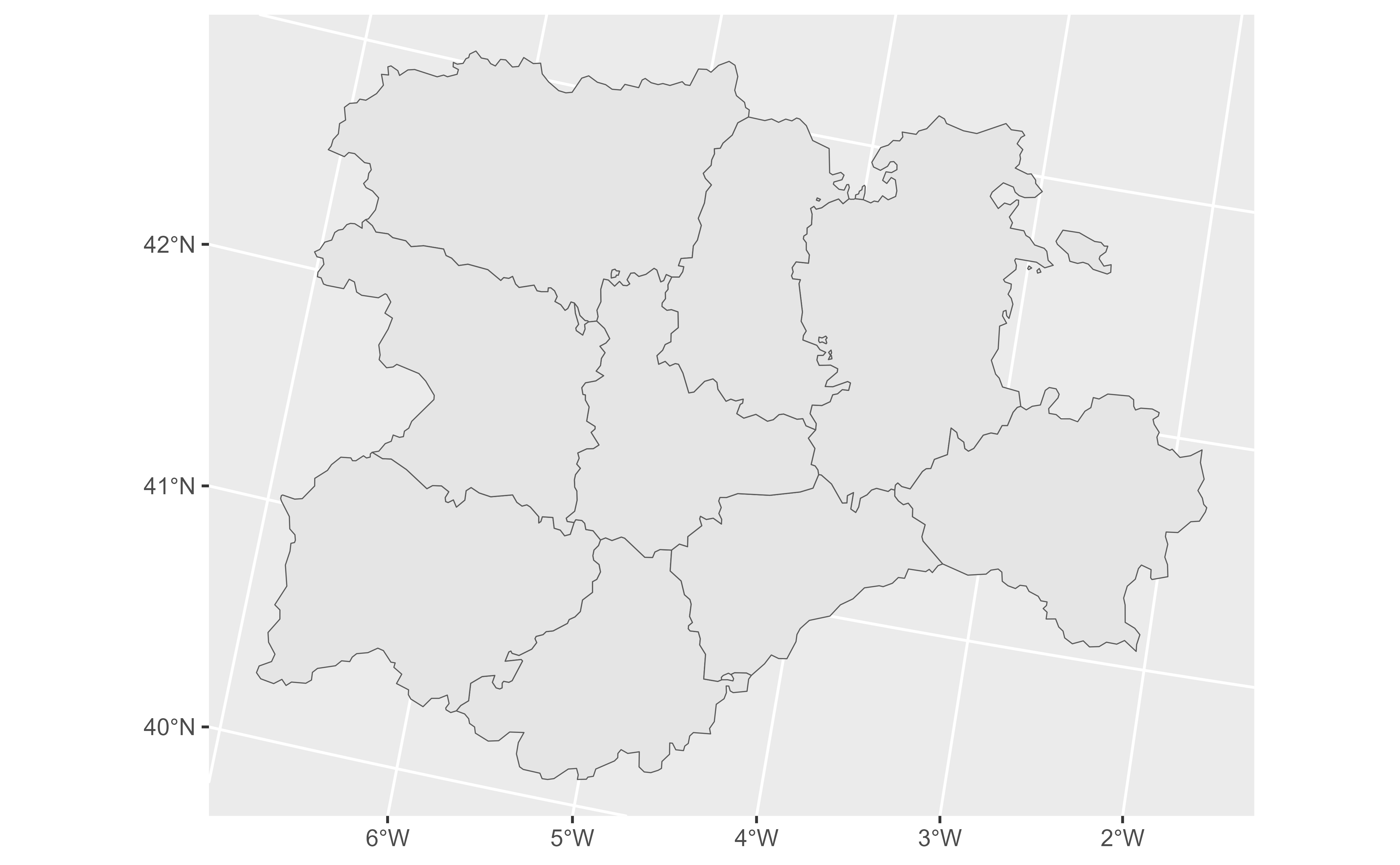
# For SpatVector, SpatGraticule and SpatExtent, use geom_sf().

# Create a SpatVector.
extfile <- system.file("extdata/cyl.gpkg", package = "tidyterra")
cyl <- terra::vect(extfile)

class(cyl)
#> [1] "SpatVector"
#> attr(,"package")
#> [1] "terra"

ggplot(cyl) +
  geom_sf()


# SpatGraticule
g <- terra::graticule(60, 30, crs = "+proj=robin")

class(g)
#> [1] "SpatGraticule"
#> attr(,"package")
#> [1] "terra"

ggplot(g) +
  geom_sf()


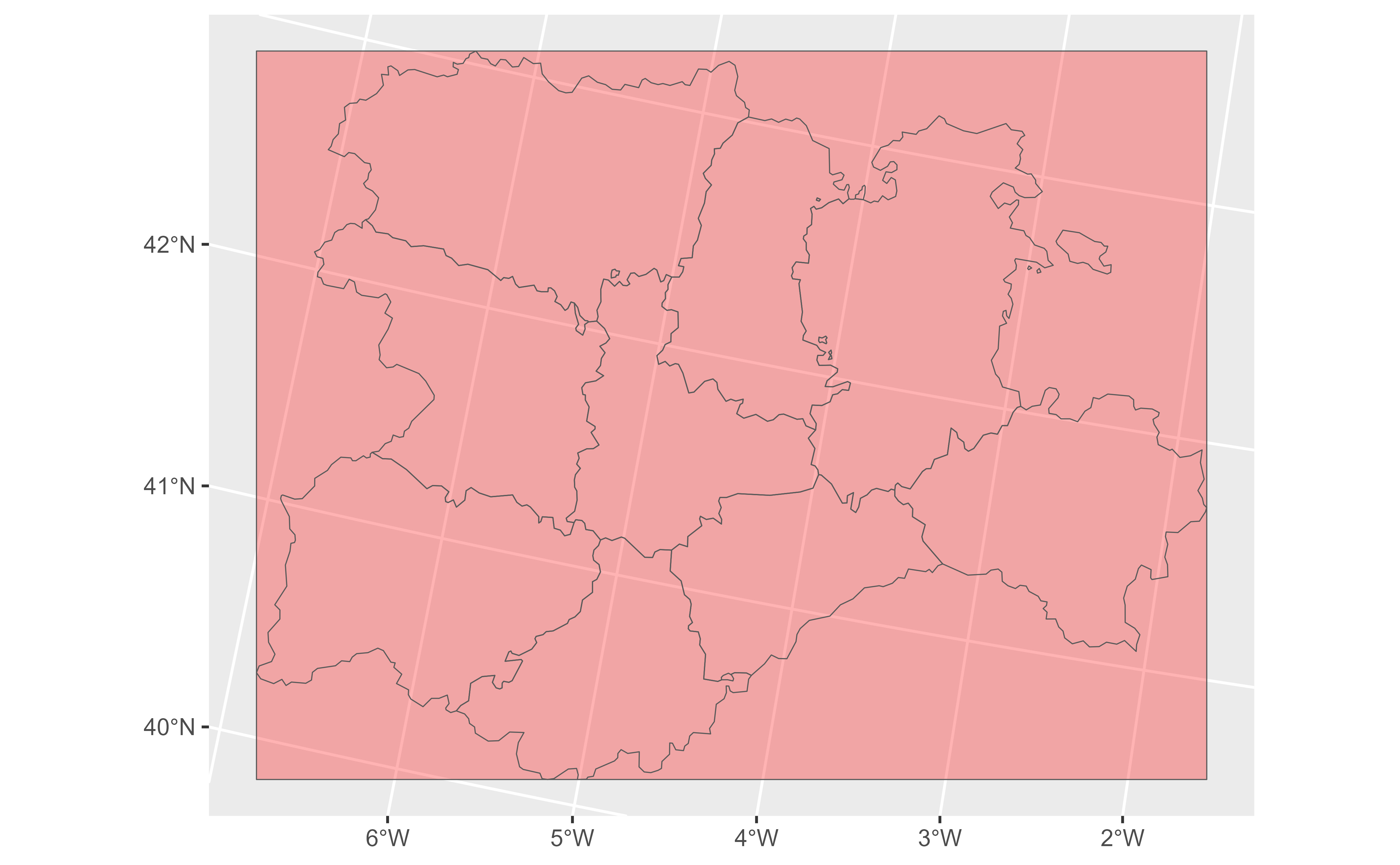
# SpatExtent
ex <- terra::ext(cyl)

class(ex)
#> [1] "SpatExtent"
#> attr(,"package")
#> [1] "terra"

ggplot(ex, crs = cyl) +
  geom_sf(fill = "red", alpha = 0.3) +
  geom_sf(data = cyl, fill = NA)

# }

Fortify `Spat*` objects