Using the tidyverse with terra objects: the tidyterra package
JOSS paper
2023-07-18
Source:vignettes/tidyterra.qmd

Summary
tidyterra is an R (R Core Team 2023) package that lets users manipulate SpatRaster and SpatVector objects provided by terra (Hijmans 2023), using verbs from packages in the tidyverse (Wickham et al. 2019), such as dplyr (Wickham, François, et al. 2023), tidyr (Wickham, Vaughan, et al. 2023) or tibble (Müller and Wickham 2023). This makes spatial data manipulation and analysis more approachable for users already familiar with the tidyverse.
tidyterra also extends ggplot2 (Wickham 2016) by providing additional geoms and stats,1 such as geom_spatraster() and geom_spatvector(), as well as carefully chosen scales and color palettes for map production.
tidyterra can manipulate the following classes of terra objects:
SpatVectorobjects, which represent vector data such as points, lines or polygon geometries.SpatRasterobjects, which represent raster data in the form of a grid consisting of equally sized cells. Each cell can contain one or more values.
The first stable version of tidyterra was released on CRAN on April 24, 2022. Since then, it has been actively used by other packages, such as ebvcube (Quoss et al. 2021), biomod2 (Thuiller et al. 2023), inlabru (Bachl et al. 2019), RCzechia (Lacko 2023) and sparrpowR (Buller et al. 2021). It has also been cited in academic research and publications (Bahlburg et al. (2023), Moraga (2024), Leonardi et al. (2023), Meister et al. (2023)).
Statement of need
The tidyverse is a collection of R packages that share an underlying design philosophy, grammar and data structures. The packages within the tidyverse are widely used by R users for tidying, transforming and plotting data.
The tidyverse is designed to work with tidy data (“every column is a variable, every row is an observation, every cell is a single value”), represented in the form of data frames or tibbles. However, it is possible to extend the functionality of tidyverse packages to work with new R object classes by registering the corresponding S3 methods (Wickham 2019). This means that dplyr::mutate() can be adapted to work with any object of class foo by creating the corresponding S3 method mutate.foo().
While other popular packages designed for spatial data handling, such as sf (Pebesma 2018) or stars (Pebesma and Bivand 2023), already provide integration with the tidyverse as part of their infrastructure, terra objects lack this integration natively. Although terra offers a wide range of functions for transforming and plotting SpatRaster and SpatVector objects, some users who are not familiar with this package may need extra time to learn that syntax. This can make their first steps in spatial analysis more difficult.
The tidyterra package was developed to address this integration gap. By providing the corresponding S3 methods, users can apply familiar syntax and functions for rectangular data to objects provided by terra. This makes spatial data analysis more approachable for users who are new to the field.
In addition, tidyterra offers functions for plotting terra objects using the ggplot2 syntax. Although packages like rasterVis (Perpiñán and Hijmans 2023) and ggspatial (Dunnington 2023) already support plotting SpatRaster objects with ggplot2, tidyterra functions provide additional support for advanced mapping. This support includes faceted maps, contours and automatic conversion of spatial layers to the same CRS2 through ggplot2::coord_sf(). tidyterra also provides support for SpatVector objects, similar to the native support of sf objects in ggplot2.
Finally, tidyterra provides a collection of color palettes specifically designed for representing spatial phenomena (Lindsay 2018). It also implements the cross-blended hypsometric tints described by Patterson and Jenny (2011).
A note on performance
The development philosophy of tidyterra is to adapt terra objects to data frame-like structures while performing data transformations, which can affect performance.
When manipulating large SpatRaster objects, such as objects with more than 10,000,000 data slots, use native terra syntax, which is designed for this type of data. For plotting, the geoms resample SpatRaster objects with more than 500,000 cells by default to speed up rendering, as terra::plot() does. You can override this upper limit with the geom’s maxcell argument.
When possible, each tidyterra help page references its equivalent terra function.
Example of use
tidyterra is available on CRAN and can be installed easily from R with:
install.packages("tidyterra")The latest development version is hosted on GitHub and can be installed from R with:
remotes::install_github("dieghernan/tidyterra")The following example demonstrates how to manipulate a SpatRaster object with dplyr syntax. It also shows how to plot a SpatRaster object with ggplot2 using geom_spatraster():
library(tidyterra)
library(tidyverse) # Load all tidyverse packages at once.
library(scales) # Additional package for labels.

# Temperatures in Castile and Leon (selected months).
rastertemp <- terra::rast(system.file(
  "extdata/cyl_temp.tif",
  package = "tidyterra"
))

# Rename with the tidyverse.
rastertemp <- rastertemp |>
  rename(April = tavg_04, May = tavg_05, June = tavg_06)

# Plot with facets.
ggplot() +
  geom_spatraster(data = rastertemp) +
  facet_wrap(~lyr, ncol = 2) +
  scale_fill_whitebox_c(
    palette = "muted",
    labels = label_number(suffix = "º"),
    n.breaks = 12,
    guide = guide_legend(reverse = TRUE)
  ) +
  labs(
    fill = "",
    title = "Average temperature in Castile and Leon (Spain)",
    subtitle = "Months of April, May and June"
  )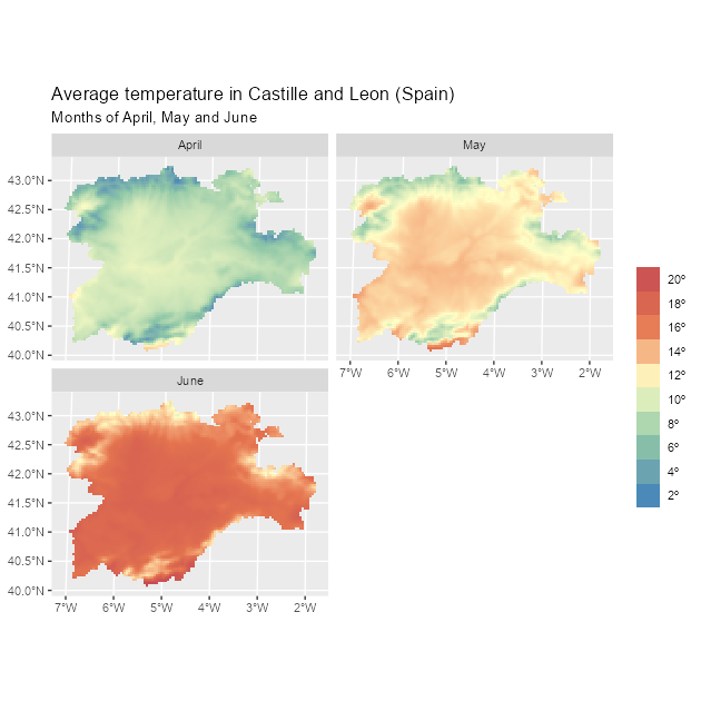
Faceted map with a multi-layer SpatRaster object.
In the following example, we combine a common dplyr workflow (mutate() + select()) and plot the result. In this case, the plot is a contour plot of the original SpatRaster using geom_spatraster_contour_filled() and includes an overlay of a SpatVector for reference:
# Compute the variation between April and June and apply a different palette.
incr_temp <- rastertemp |>
  mutate(var = June - April) |>
  select(Variation = var)

# Overlay a SpatVector.
cyl_vect <- terra::vect(system.file("extdata/cyl.gpkg", package = "tidyterra"))

# Contour map with overlay.
ggplot() +
  geom_spatraster_contour_filled(data = incr_temp) +
  geom_spatvector(data = cyl_vect, fill = NA) +
  scale_fill_whitebox_d(palette = "bl_yl_rd") +
  theme_grey() +
  labs(
    fill = "º Celsius",
    title = "Temperature variation in Castile and Leon (Spain)",
    subtitle = "Difference between April and June"
  )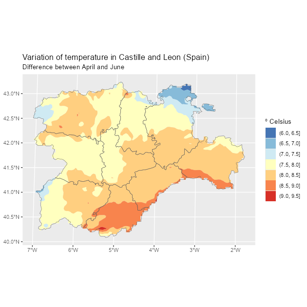
Contour map of temperature variation with a SpatVector overlay.
Additional materials
The package includes extensive documentation available online at https://dieghernan.github.io/tidyterra/ including:
- Details on each function, including the equivalent terra function when available, for users who prefer to include those functions in their workflows.
- Working examples that use the functions and create plots.
- Additional articles and vignettes, including a complete demo of the color palettes included in the package (see Palettes).
Acknowledgements
I would like to thank Robert J. Hijmans for his advice and support in adapting some of the methods and for the suggestions that helped us improve the package features. I am also thankful to Dewey Dunnington, Brent Thorne and the rest of the contributors to the ggspatial package, which served as a key reference during the initial stages of the development of tidyterra.
tidyterra also incorporates some pieces of code adapted from ggplot2 for computing contours, which relies on the package isoband (Wickham et al. 2022) developed by Claus O. Wilke.