Welcome to tidyterra

tidyterra

tidyterra provides methods from tidyverse packages for SpatRaster and SpatVector objects created with terra. It also provides geom_spat*() geoms and scales for plotting those objects with ggplot2.

Why tidyterra?

Spat* objects differ from regular data frames: they are S4 objects with their own syntax and computational methods (implemented in terra). By providing tidyverse verbs, especially dplyr and tidyr methods, tidyterra lets users manipulate Spat* objects in a style familiar from tabular data workflows.

terra is generally faster. Learning some terra syntax is recommended because tidyterra functions call the corresponding terra equivalents when possible.

A note for advanced terra users

tidyterra is not optimized for performance. Operations such as filter() and mutate() can be slower than their terra counterparts.

As a rule of thumb, tidyterra is most suitable for objects with fewer than 10,000,000 data slots, for example terra::ncell(a_rast) * terra::nlyr(a_rast) < 1e7.

Get started with tidyterra

Load tidyterra together with core tidyverse packages:

library(tidyterra)
library(dplyr)
library(tidyr)

The following methods are available:

tidyverse method	`SpatVector`	`SpatRaster`
`tibble::as_tibble()`	✔️	✔️
`dplyr::select()`	✔️	✔️ Select layers
`dplyr::mutate()`	✔️	✔️ Create or modify layers
`dplyr::transmute()`	✔️	✔️
`dplyr::filter()`	✔️	✔️ Modify cell values and optionally remove outer cells.
`dplyr::filter_out()`	✔️
`dplyr::slice()`	✔️	✔️ Additional methods for slicing by row and column.
`dplyr::pull()`	✔️	✔️
`dplyr::rename()`	✔️	✔️
`dplyr::relocate()`	✔️	✔️
`dplyr::distinct()`	✔️
`dplyr::arrange()`	✔️
`dplyr::glimpse()`	✔️	✔️
`dplyr::inner_join()` family	✔️
`dplyr::nest_join()`	✔️
`dplyr::cross_join()`	✔️
`dplyr::summarise()`	✔️
`dplyr::reframe()`	✔️
`dplyr::group_by()` family	✔️
`dplyr::rowwise()`	✔️
`dplyr::count()`, `tally()`	✔️
`dplyr::add_count()`	✔️
`dplyr::rows_*()`	✔️
`dplyr::bind_cols()` / `dplyr::bind_rows()`	✔️ as `bind_spat_cols()` / `bind_spat_rows()`
`tidyr::drop_na()`	✔️	✔️ Remove cell values with `NA` on any layer and outer cells with `NA`.
`tidyr::complete()`	✔️
`tidyr::expand()`	✔️
`tidyr::replace_na()`	✔️	✔️
`tidyr::fill()`	✔️
`tidyr::nest()`	✔️
`tidyr::pivot_longer()`	✔️
`tidyr::pivot_wider()`	✔️
`tidyr::uncount()`	✔️
`tidyr::unite()`	✔️	✔️ Create a categorical layer.
`ggplot2::autoplot()`	✔️	✔️
`ggplot2::fortify()`	✔️ to sf through `sf::st_as_sf()`	To a tibble with coordinates.
`ggplot2::geom_*()`	✔️ `geom_spatvector()`	✔️ `geom_spatraster()` and `geom_spatraster_rgb()`.
`generics::tidy()`	✔️	✔️
`generics::glance()`	✔️	✔️
`generics::required_pkgs()`	✔️	✔️

The following sections show some of these methods in action.

`SpatRaster` objects

This example uses a SpatRaster:

library(terra)
f <- system.file("extdata/cyl_temp.tif", package = "tidyterra")

temp <- rast(f)

temp
#> class       : SpatRaster
#> size        : 87, 118, 3  (nrow, ncol, nlyr)
#> resolution  : 3881.255, 3881.255  (x, y)
#> extent      : -612335.4, -154347.3, 4283018, 4620687  (xmin, xmax, ymin, ymax)
#> coord. ref. : World_Robinson (ESRI:54030)
#> source      : cyl_temp.tif
#> names       :   tavg_04,   tavg_05,   tavg_06
#> min values  :  1.885463,  5.817587, 10.463377
#> max values  : 13.283829, 16.740898, 21.113781

mod <- temp |>
  select(-1) |>
  mutate(newcol = tavg_06 - tavg_05) |>
  relocate(newcol, .before = 1) |>
  replace_na(list(newcol = 3)) |>
  rename(difference = newcol)

mod
#> class       : SpatRaster
#> size        : 87, 118, 3  (nrow, ncol, nlyr)
#> resolution  : 3881.255, 3881.255  (x, y)
#> extent      : -612335.4, -154347.3, 4283018, 4620687  (xmin, xmax, ymin, ymax)
#> coord. ref. : World_Robinson (ESRI:54030)
#> source(s)   : memory
#> names       : difference,   tavg_05,   tavg_06
#> min values  :   2.817647,  5.817587, 10.463377
#> max values  :   5.307511, 16.740898, 21.113781

In this example we:

Removed the first layer (tavg_04).
Created a new layer newcol as the difference between tavg_06 and tavg_05.
Relocated newcol to be the first layer.
Replaced NA values in newcol with 3.
Renamed newcol to difference.

Throughout these steps, core properties of the SpatRaster, including number of cells, rows, columns, extent, resolution and CRS, remain unchanged. Other verbs such as filter(), slice() or drop_na() may alter these properties in a manner analogous to row operations on data frames.

`SpatVector` objects

Most dplyr and tidyr verbs work with SpatVector objects, so you can arrange, group and summarize their attributes.

lux <- system.file("ex/lux.shp", package = "terra")

v_lux <- vect(lux)

v_lux |>
  # Create categories.
  mutate(gr = cut(POP / 1000, 5)) |>
  group_by(gr) |>
  # Summarize by group.
  summarise(
    n = n(),
    tot_pop = sum(POP),
    mean_area = mean(AREA)
  ) |>
  # Arrange groups.
  arrange(desc(gr))
#> class       : SpatVector
#> geometry    : polygons
#> dimensions  : 3, 4  (geometries, attributes)
#> extent      : 5.74414, 6.528252, 49.44781, 50.18162  (xmin, xmax, ymin, ymax)
#> coord. ref. : lon/lat WGS 84 (EPSG:4326)
#> names       :          gr     n tot_pop mean_area
#> type        :      <fact> <int>   <num>     <num>
#> values      :   (147,183]     2  359427       244
#>               (40.7,76.1]     1   48187       185
#>               (4.99,40.7]     9  194391   209.778

As with SpatRaster, essential properties such as geometry and CRS are preserved during these operations.

Plotting with ggplot2

`SpatRaster` objects

When a SpatRaster has a CRS defined (terra::crs(a_rast) != ""), the geom uses ggplot2::coord_sf() and can reproject the raster to match other spatial layers.

library(ggplot2)

# Facet a SpatRaster object.

ggplot() +
  geom_spatraster(data = temp) +
  facet_wrap(~lyr) +
  scale_fill_whitebox_c(
    palette = "muted",
    na.value = "white"
  )

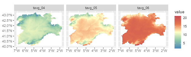
Faceted map using a SpatRaster object.

# Contour lines for a specific layer.

f_volcano <- system.file("extdata/volcano2.tif", package = "tidyterra")
volcano2 <- rast(f_volcano)

ggplot() +
  geom_spatraster(data = volcano2) +
  geom_spatraster_contour(data = volcano2, breaks = seq(80, 200, 5)) +
  scale_fill_whitebox_c() +
  coord_sf(expand = FALSE) +
  labs(fill = "elevation")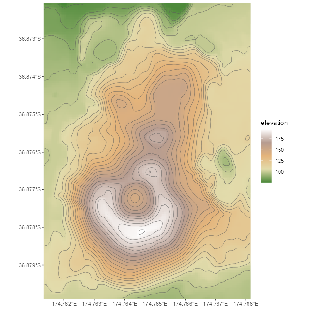

Contour line plot for a SpatRaster object.

# Filled contours.

ggplot() +
  geom_spatraster_contour_filled(data = volcano2) +
  scale_fill_whitebox_d(palette = "atlas") +
  labs(fill = "elevation")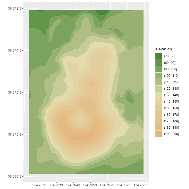

Filled contour plot for a SpatRaster object.

tidyterra also supports RGB SpatRaster objects for imagery:

# Read a vector.

f_v <- system.file("extdata/cyl.gpkg", package = "tidyterra")
v <- vect(f_v)

# Read a tile.
f_rgb <- system.file("extdata/cyl_tile.tif", package = "tidyterra")

r_rgb <- rast(f_rgb)

rgb_plot <- ggplot(v) +
  geom_spatraster_rgb(data = r_rgb) +
  geom_spatvector(fill = NA, size = 1)

rgb_plot

Map combining an RGB SpatRaster object and a SpatVector object.

tidyterra includes color scales and hypsometric tints suitable for topographic and bathymetric maps:

asia <- rast(system.file("extdata/asia.tif", package = "tidyterra"))

asia
#> class       : SpatRaster
#> size        : 164, 306, 1  (nrow, ncol, nlyr)
#> resolution  : 31836.23, 31847.57  (x, y)
#> extent      : 7619120, 1.736101e+07, -1304745, 3918256  (xmin, xmax, ymin, ymax)
#> coord. ref. : WGS 84 / Pseudo-Mercator (EPSG:3857)
#> source      : asia.tif
#> name        : file44bc291153f2
#> min value   :     -9558.467773
#> max value   :      5801.927246

ggplot() +
  geom_spatraster(data = asia) +
  scale_fill_hypso_tint_c(
    palette = "gmt_globe",
    labels = scales::label_number(),
    # Further refinements
    breaks = c(-10000, -5000, 0, 2000, 5000, 8000),
    guide = guide_colorbar(reverse = TRUE)
  ) +
  labs(
    fill = "elevation (m)",
    title = "Hypsometric map of Asia"
  ) +
  theme(
    legend.position = "bottom",
    legend.title.position = "top",
    legend.key.width = rel(3),
    legend.ticks = element_line(colour = "black", linewidth = 0.3),
    legend.direction = "horizontal"
  )

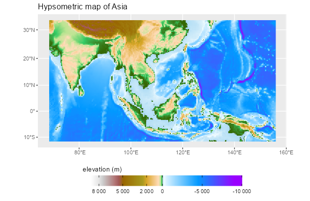
Map of Asia including hypsometric tints.

`SpatVector` objects

Plot SpatVector objects with geom_spatvector():

lux <- system.file("ex/lux.shp", package = "terra")

v_lux <- terra::vect(lux)

ggplot(v_lux) +
  geom_spatvector(aes(fill = POP), color = "white") +
  geom_spatvector_text(aes(label = NAME_2), color = "grey90") +
  scale_fill_binned(labels = scales::number_format()) +
  coord_sf(crs = 3857)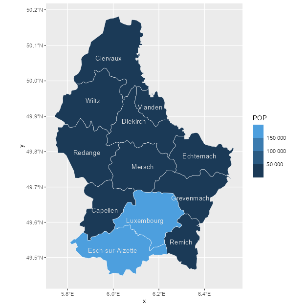

Choropleth map with a SpatVector object.

Internally, tidyterra converts terra::vect() output to sf with sf::st_as_sf() and then uses ggplot2::geom_sf() to render the layer.

You can also aggregate SpatVector objects easily:

# Dissolve by group.
v_lux |>
  # Create categories.
  mutate(gr = cut(POP / 1000, 5)) |>
  group_by(gr) |>
  # Summarize by group.
  summarise(
    n = n(),
    tot_pop = sum(POP),
    mean_area = mean(AREA)
  ) |>
  ggplot() +
  geom_spatvector(aes(fill = tot_pop), color = "black") +
  geom_spatvector_label(aes(label = gr)) +
  coord_sf(crs = 3857)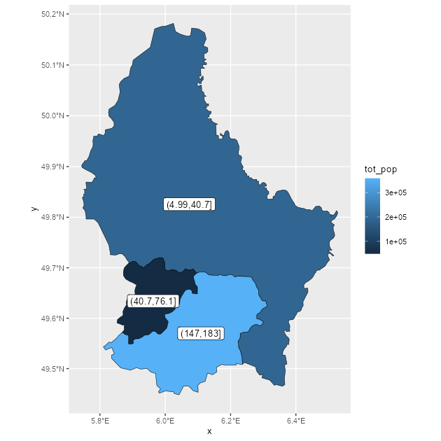

Dissolving SpatVector objects by group.


# Repeat while keeping internal boundaries.
v_lux |>
  # Create categories.
  mutate(gr = cut(POP / 1000, 5)) |>
  group_by(gr) |>
  # Summarize by group without dissolving.
  summarise(
    n = n(),
    tot_pop = sum(POP),
    mean_area = mean(AREA),
    .dissolve = FALSE
  ) |>
  ggplot() +
  geom_spatvector(aes(fill = tot_pop), color = "black") +
  geom_spatvector_label(aes(label = gr)) +
  coord_sf(crs = 3857)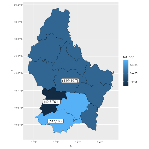

Dissolving SpatVector objects by group, keeping internal boundaries.

tidyterra

Why tidyterra?

A note for advanced terra users

Get started with tidyterra

SpatRaster objects

SpatVector objects

Plotting with ggplot2

SpatRaster objects

SpatVector objects

`SpatRaster` objects

`SpatVector` objects

`SpatRaster` objects

`SpatVector` objects