Implementation of GRASS color tables. The following fill scales and palettes are provided:
scale_*_grass_d(): For discrete values.scale_*_grass_c(): For continuous values.scale_*_grass_b(): For binning continuous values.grass.colors(): Gradient color palette. See alsogrDevices::terrain.colors()for details.
Additional arguments ... are passed to:
Discrete values:
ggplot2::discrete_scale().Continuous values:
ggplot2::continuous_scale().Binned continuous values:
ggplot2::binned_scale().
tidyterra documents only a subset of these additional arguments, so see the ggplot2 functions listed above for the full range.
These palettes implement terra::map.pal(), the default color palettes used
by terra::plot() in terra versions above 1.7.78.
Usage
scale_fill_grass_d(
  palette = "viridis",
  ...,
  alpha = 1,
  direction = 1,
  na.translate = FALSE,
  drop = TRUE
)

scale_colour_grass_d(
  palette = "viridis",
  ...,
  alpha = 1,
  direction = 1,
  na.translate = FALSE,
  drop = TRUE
)

scale_fill_grass_c(
  palette = "viridis",
  ...,
  alpha = 1,
  direction = 1,
  values = NULL,
  limits = NULL,
  use_grass_range = TRUE,
  na.value = "transparent",
  guide = "colourbar"
)

scale_colour_grass_c(
  palette = "viridis",
  ...,
  alpha = 1,
  direction = 1,
  values = NULL,
  limits = NULL,
  use_grass_range = TRUE,
  na.value = "transparent",
  guide = "colourbar"
)

scale_fill_grass_b(
  palette = "viridis",
  ...,
  alpha = 1,
  direction = 1,
  values = NULL,
  limits = NULL,
  use_grass_range = TRUE,
  na.value = "transparent",
  guide = "coloursteps"
)

scale_colour_grass_b(
  palette = "viridis",
  ...,
  alpha = 1,
  direction = 1,
  values = NULL,
  limits = NULL,
  use_grass_range = TRUE,
  na.value = "transparent",
  guide = "coloursteps"
)

grass.colors(n, palette = "viridis", alpha = 1, rev = FALSE)
Source
Derived from https://github.com/OSGeo/grass/tree/main/lib/gis/colors. See also r.color - GRASS GIS Manual.
Arguments
- palette
A valid palette name. The name is matched to the list of available palettes, ignoring upper vs. lower case. See grass_db for more information.
- ...
Arguments passed on to
ggplot2::discrete_scale,ggplot2::continuous_scale,ggplot2::binned_scalebreaksOne of:
minor_breaksOne of:
NULLfor no minor breakswaiver()for the default breaks (none for discrete, one minor break between each major break for continuous)A numeric vector of positions
A function that given the limits returns a vector of minor breaks. Also accepts rlang lambda function notation. When the function has two arguments, it will be given the limits and major break positions.
labelsOne of the options below. Please note that when
labelsis a vector, it is highly recommended to also set thebreaksargument as a vector to protect against unintended mismatches.NULLfor no labelswaiver()for the default labels computed by the transformation objectA character vector giving labels (must be same length as
breaks)An expression vector (must be the same length as breaks). See ?plotmath for details.
A function that takes the breaks as input and returns labels as output. Also accepts rlang lambda function notation.
expandFor position scales, a vector of range expansion constants used to add some padding around the data to ensure that they are placed some distance away from the axes. Use the convenience function
expansion()to generate the values for theexpandargument. The defaults are to expand the scale by 5% on each side for continuous variables, and by 0.6 units on each side for discrete variables.n.breaksAn integer guiding the number of major breaks. The algorithm may choose a slightly different number to ensure nice break labels. Will only have an effect if
breaks = waiver(). UseNULLto use the default number of breaks given by the transformation.nice.breaksLogical. Should breaks be attempted placed at nice values instead of exactly evenly spaced between the limits. If
TRUE(default) the scale will ask the transformation object to create breaks, and this may result in a different number of breaks than requested. Ignored if breaks are given explicitly.
- alpha
The alpha transparency, a number in [0,1], see argument alpha in
hsv.- direction
Sets the order of colors in the scale. If 1, the default, colors are ordered from darkest to lightest. If -1, the order of colors is reversed.
- na.translate
Logical. If
TRUE, removeNAvalues from the legend. The default isTRUE.- drop
Logical. If
TRUE, omit unused factor levels from the scale. The default (TRUE) removes unused factors.- values
if colours should not be evenly positioned along the gradient this vector gives the position (between 0 and 1) for each colour in the
coloursvector. Seerescale()for a convenience function to map an arbitrary range to between 0 and 1.- limits
One of:
NULLto use the default scale rangeA numeric vector of length two providing limits of the scale. Use
NAto refer to the existing minimum or maximumA function that accepts the existing (automatic) limits and returns new limits. Also accepts rlang lambda function notation. Note that setting limits on positional scales will remove data outside of the limits. If the purpose is to zoom, use the limit argument in the coordinate system (see
coord_cartesian()).
- use_grass_range
Logical. If
TRUE, use the suggested range when plotting. See Details.- na.value
Missing values will be replaced with this value. By default, tidyterra uses
na.value = "transparent"so cells withNAare not filled. See also #120.- guide
A function used to create a guide or its name. See
guides()for more information.- n
the number of colors (\(\ge 1\)) to be in the palette.
- rev
logical indicating whether the ordering of the colors should be reversed.
Details
Some palettes are mapped by default to a specific range of values (see
grass_db). Set use_grass_range = FALSE to map the color scales to the
range of values of the fill/colour aesthetics. See Examples.
When passing the limits argument, the colors are restricted to those
specified by this argument, keeping the distribution of the palette. You can
combine this with oob, for example oob = scales::oob_squish, to avoid
blank pixels in the plot.
terra equivalent
References
GRASS Development Team (2024). Geographic Resources Analysis Support System (GRASS) Software, Version 8.3.2. Open Source Geospatial Foundation, USA. https://grass.osgeo.org.
See also
grass_db, terra::plot(), terra::minmax(),
ggplot2::scale_fill_viridis_c().
See also ggplot2 docs on additional ... arguments:
Other color scales, palettes and hypsometric tints:
scale_coltab,
scale_cross_blended,
scale_hypso,
scale_princess,
scale_terrain,
scale_whitebox,
scale_wiki
Examples
# \donttest{
filepath <- system.file("extdata/volcano2.tif", package = "tidyterra")
library(terra)
volcano2_rast <- rast(filepath)
# Palette
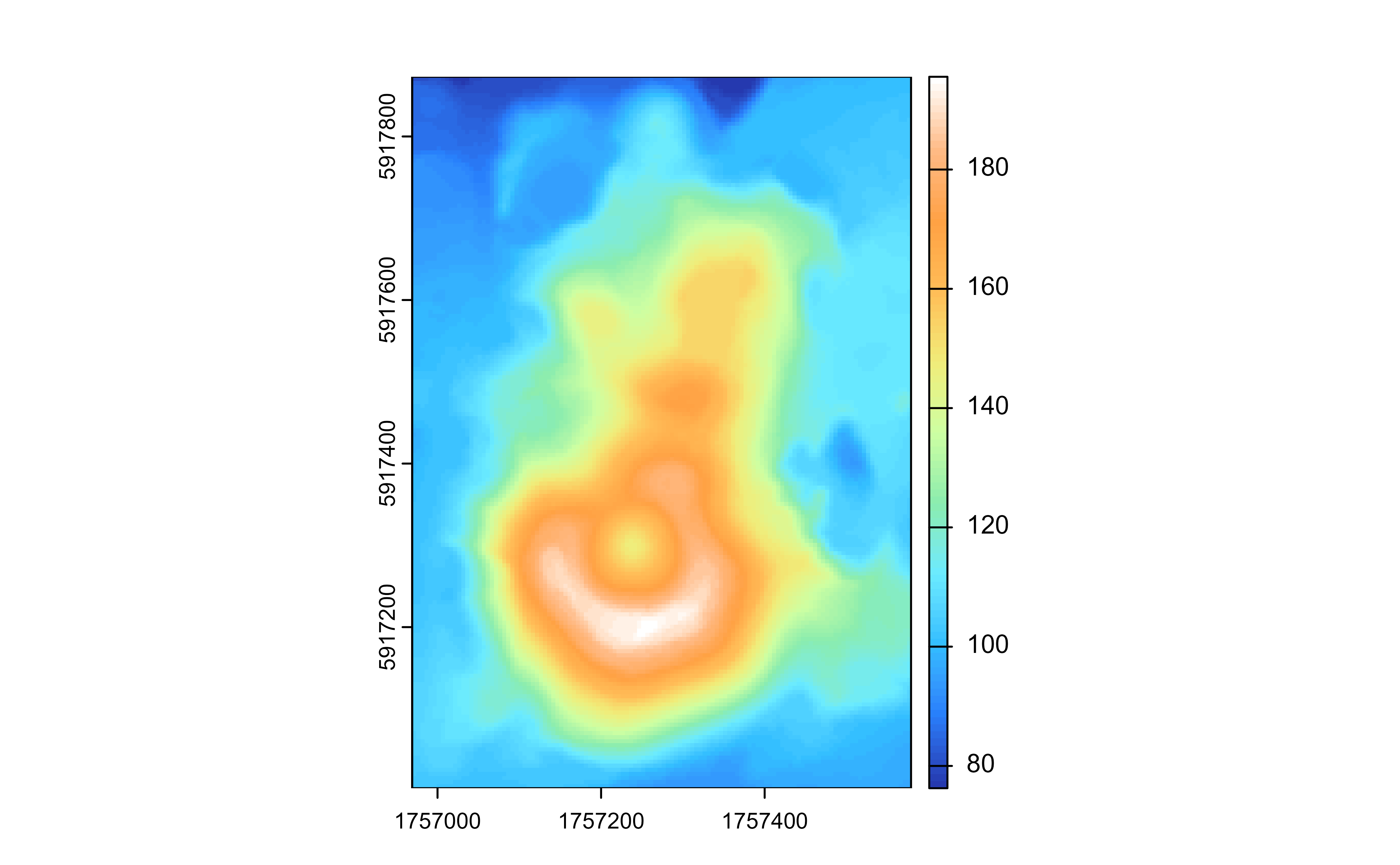
plot(volcano2_rast, col = grass.colors(100, palette = "haxby"))
 library(ggplot2)
ggplot() +
geom_spatraster(data = volcano2_rast) +
scale_fill_grass_c(palette = "terrain")
library(ggplot2)
ggplot() +
geom_spatraster(data = volcano2_rast) +
scale_fill_grass_c(palette = "terrain")
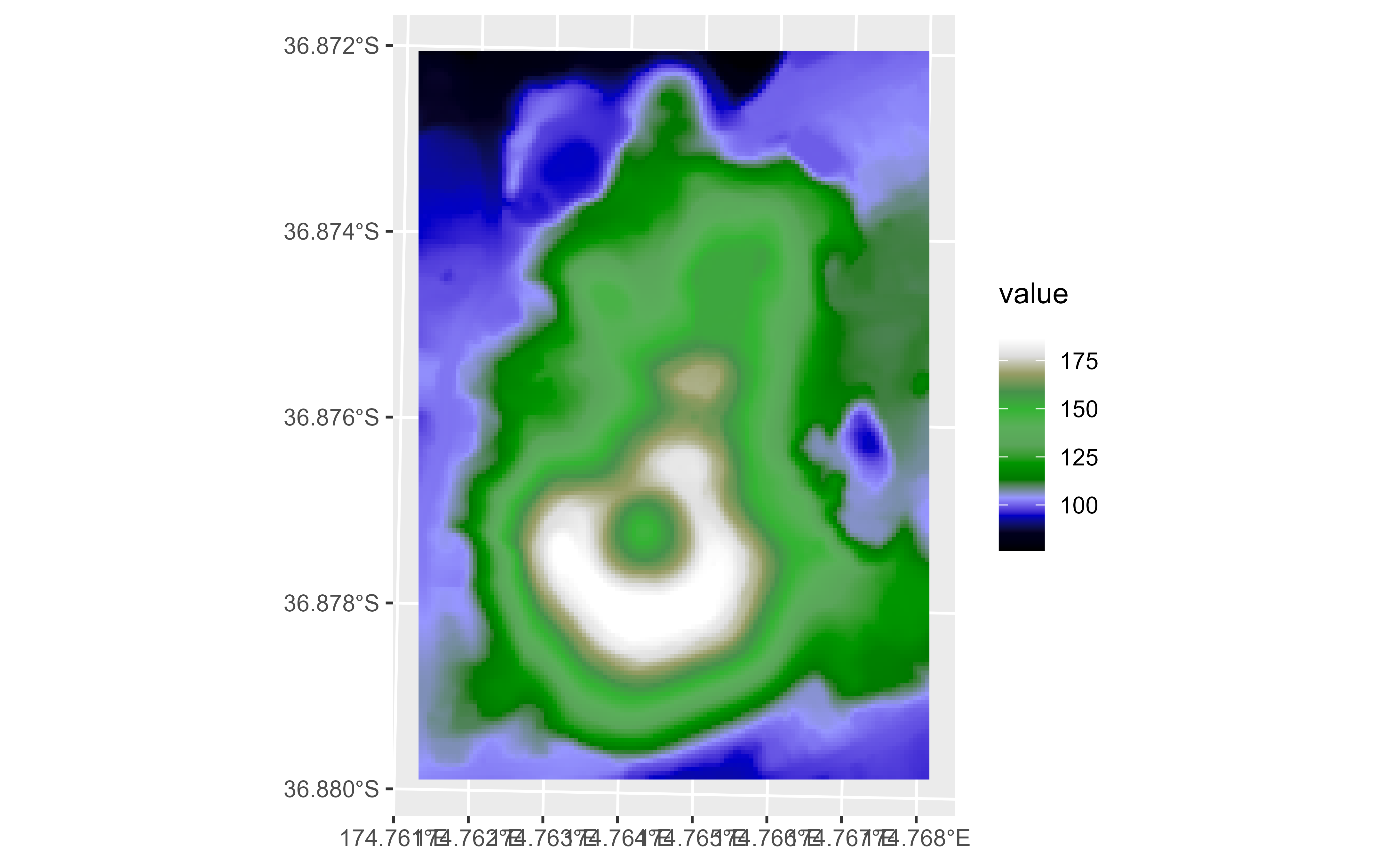
 # Use without default limits.
ggplot() +
geom_spatraster(data = volcano2_rast) +
scale_fill_grass_c(palette = "terrain", use_grass_range = FALSE)
# Use without default limits.
ggplot() +
geom_spatraster(data = volcano2_rast) +
scale_fill_grass_c(palette = "terrain", use_grass_range = FALSE)
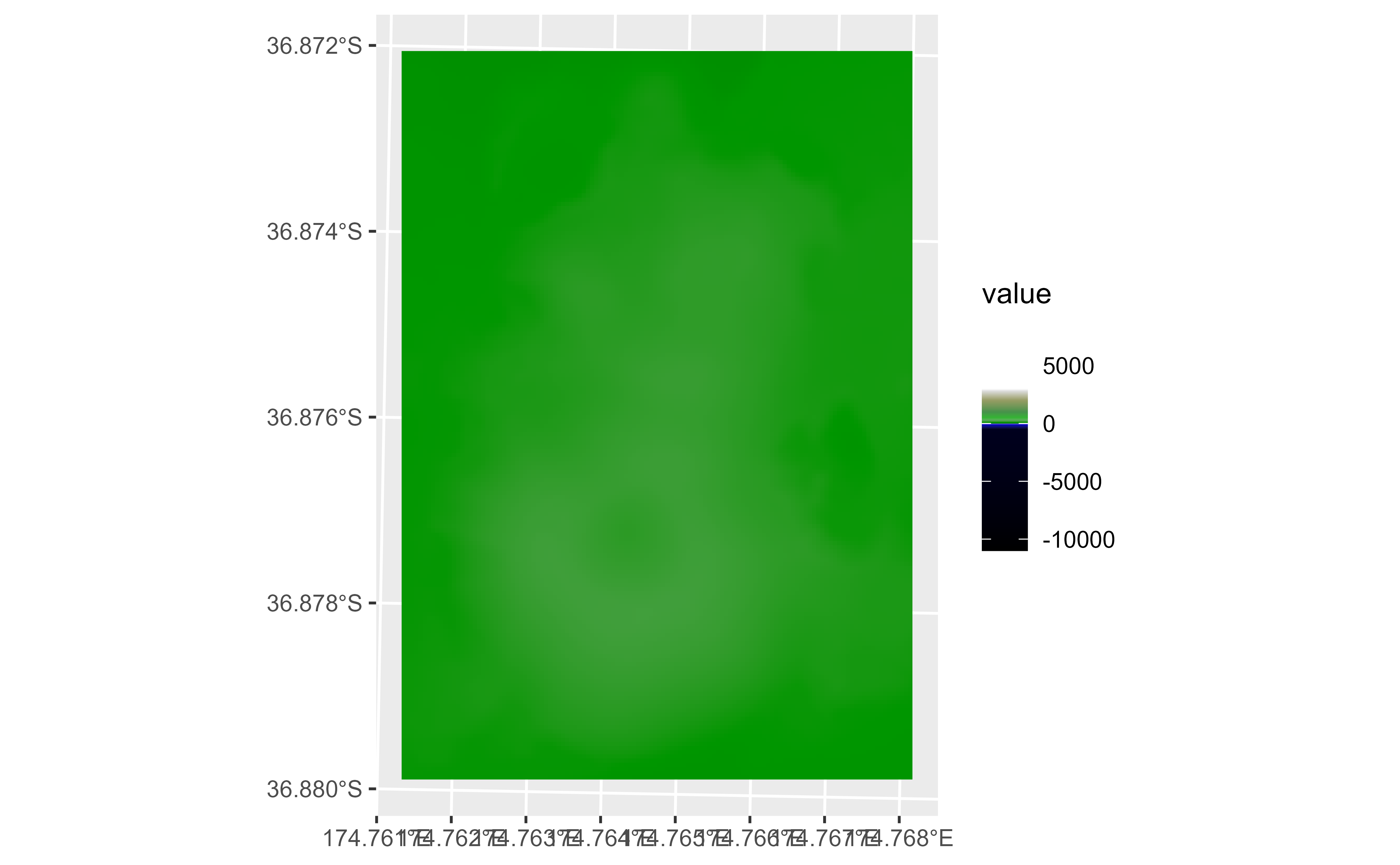
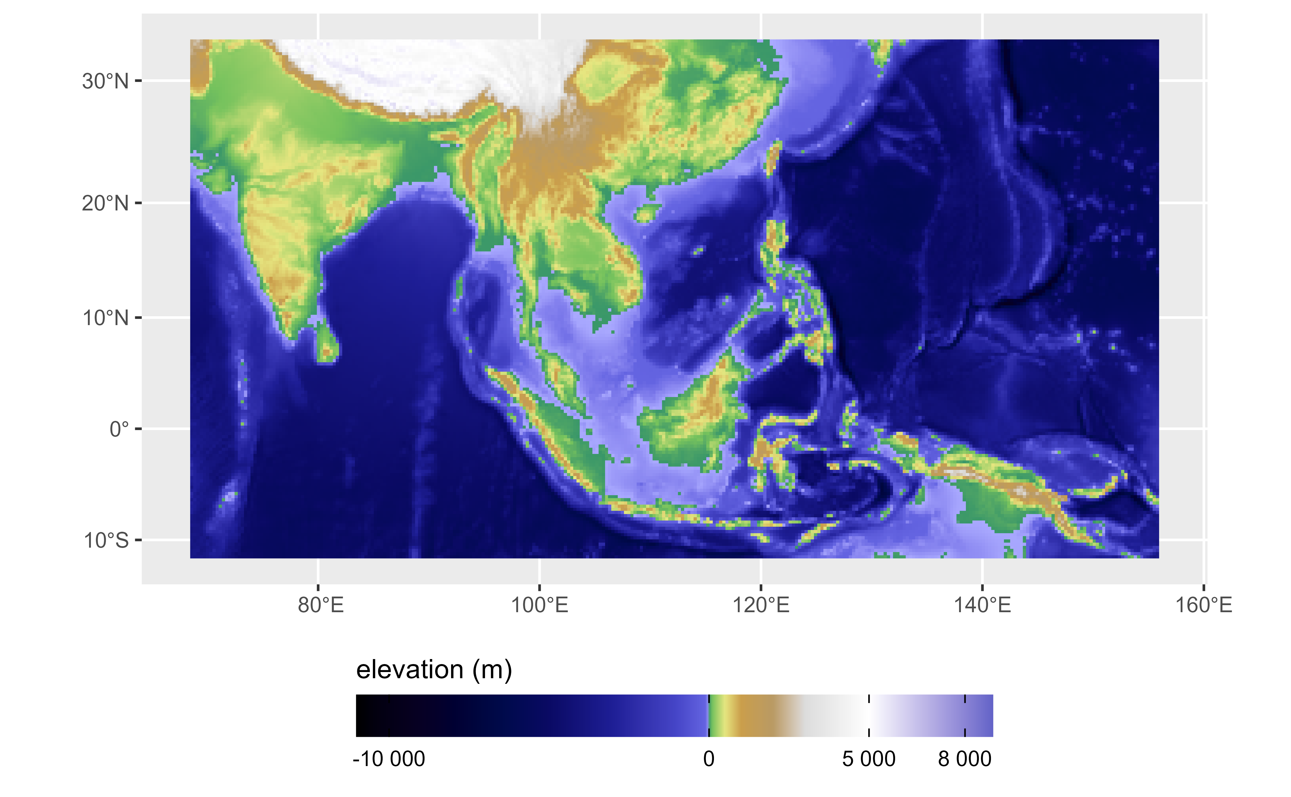
 # Full map with true tints
f_asia <- system.file("extdata/asia.tif", package = "tidyterra")
asia <- rast(f_asia)
ggplot() +
geom_spatraster(data = asia) +
scale_fill_grass_c(
palette = "srtm_plus",
labels = scales::label_number(),
breaks = c(-10000, 0, 5000, 8000),
guide = guide_colorbar(reverse = FALSE)
) +
labs(fill = "elevation (m)") +
theme(
legend.position = "bottom",
legend.title.position = "top",
legend.key.width = rel(3),
legend.ticks = element_line(colour = "black", linewidth = 0.3),
legend.direction = "horizontal"
)
# Full map with true tints
f_asia <- system.file("extdata/asia.tif", package = "tidyterra")
asia <- rast(f_asia)
ggplot() +
geom_spatraster(data = asia) +
scale_fill_grass_c(
palette = "srtm_plus",
labels = scales::label_number(),
breaks = c(-10000, 0, 5000, 8000),
guide = guide_colorbar(reverse = FALSE)
) +
labs(fill = "elevation (m)") +
theme(
legend.position = "bottom",
legend.title.position = "top",
legend.key.width = rel(3),
legend.ticks = element_line(colour = "black", linewidth = 0.3),
legend.direction = "horizontal"
)
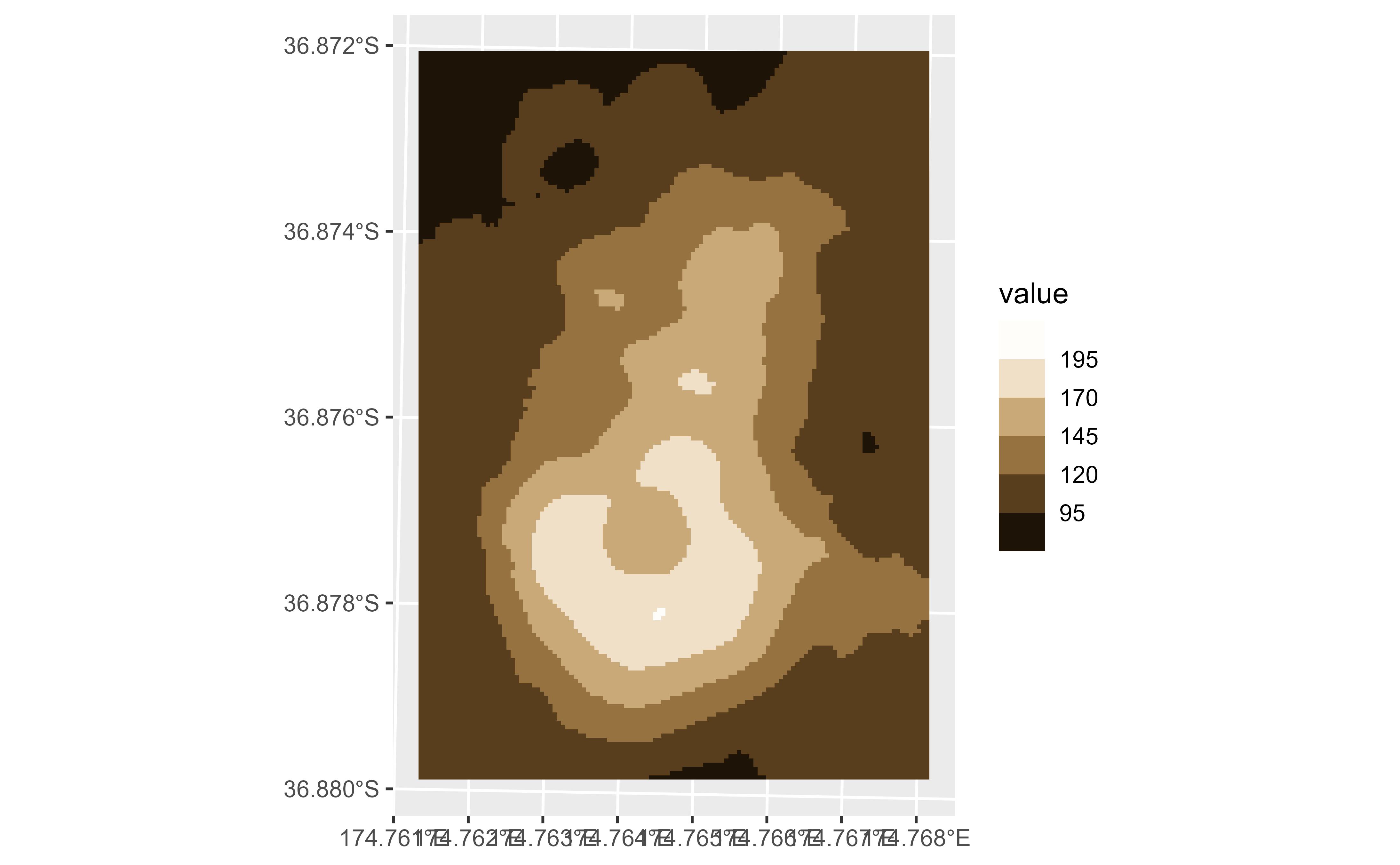
 # Binned
ggplot() +
geom_spatraster(data = volcano2_rast) +
scale_fill_grass_b(breaks = seq(70, 200, 25), palette = "sepia")
# Binned
ggplot() +
geom_spatraster(data = volcano2_rast) +
scale_fill_grass_b(breaks = seq(70, 200, 25), palette = "sepia")
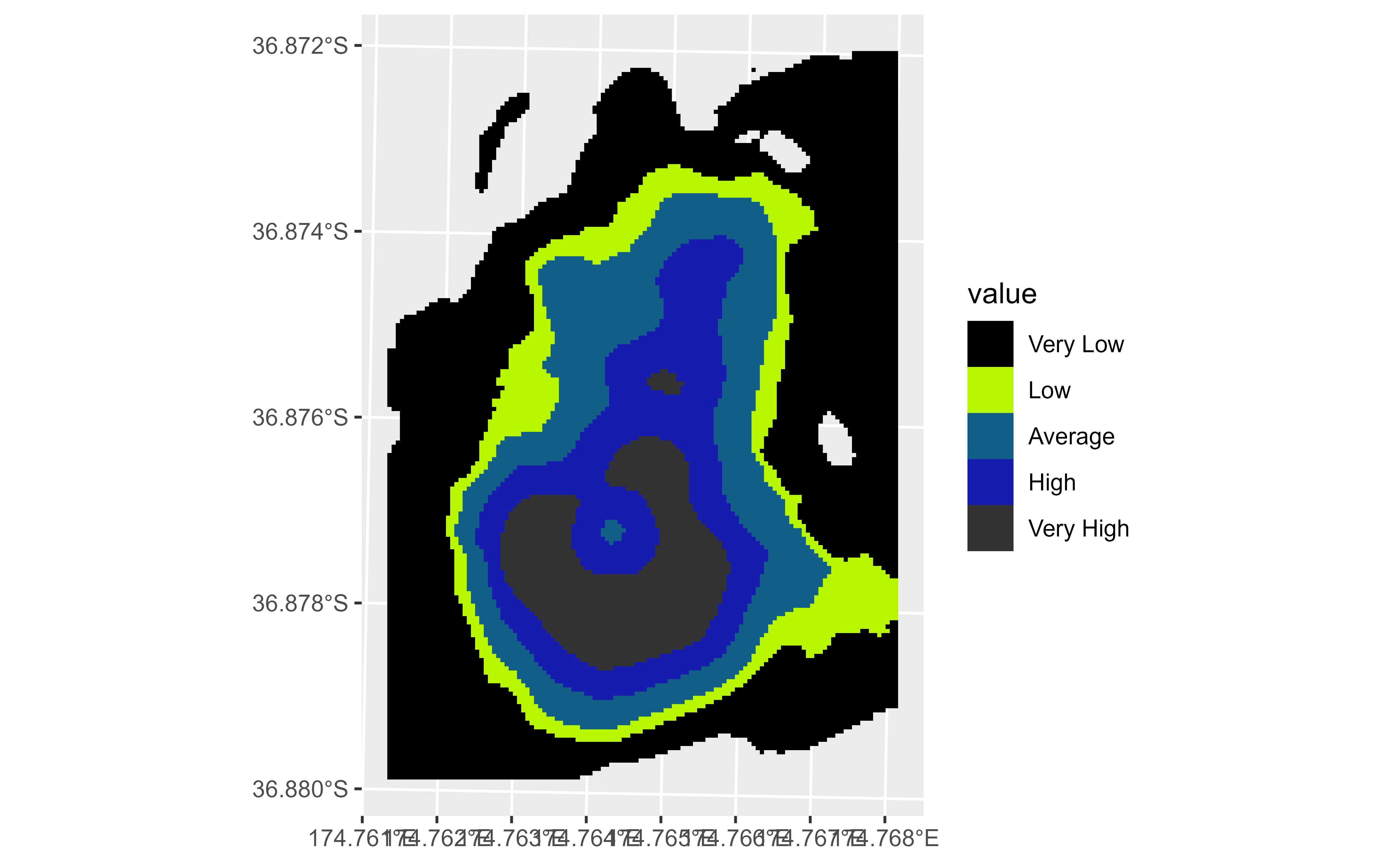
 # With discrete values
factor <- volcano2_rast |>
mutate(cats = cut(elevation,
breaks = c(100, 120, 130, 150, 170, 200),
labels = c(
"Very Low", "Low", "Average", "High",
"Very High"
)
))
ggplot() +
geom_spatraster(data = factor, aes(fill = cats)) +
scale_fill_grass_d(palette = "soilmoisture")
# With discrete values
factor <- volcano2_rast |>
mutate(cats = cut(elevation,
breaks = c(100, 120, 130, 150, 170, 200),
labels = c(
"Very Low", "Low", "Average", "High",
"Very High"
)
))
ggplot() +
geom_spatraster(data = factor, aes(fill = cats)) +
scale_fill_grass_d(palette = "soilmoisture")
 # }
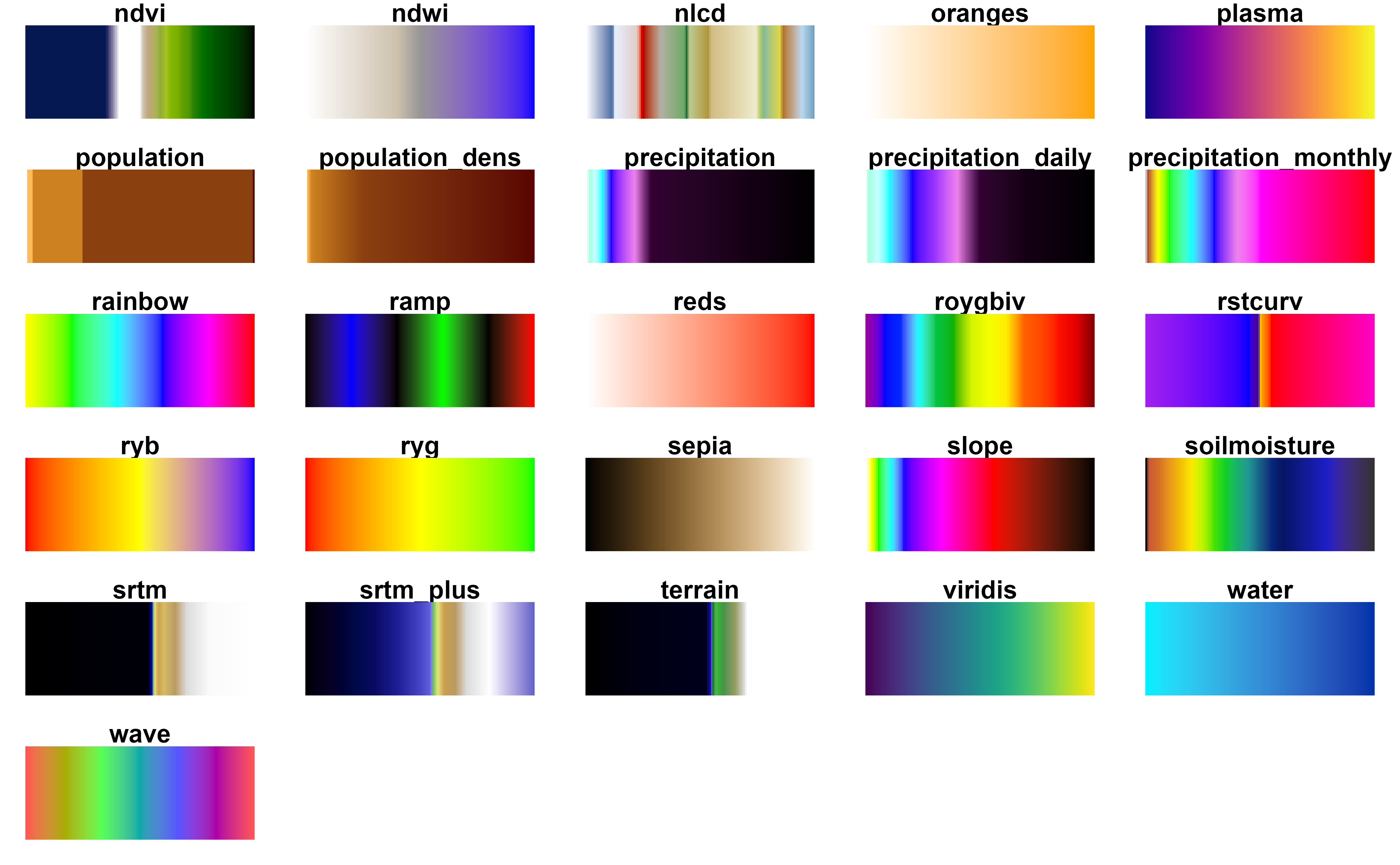
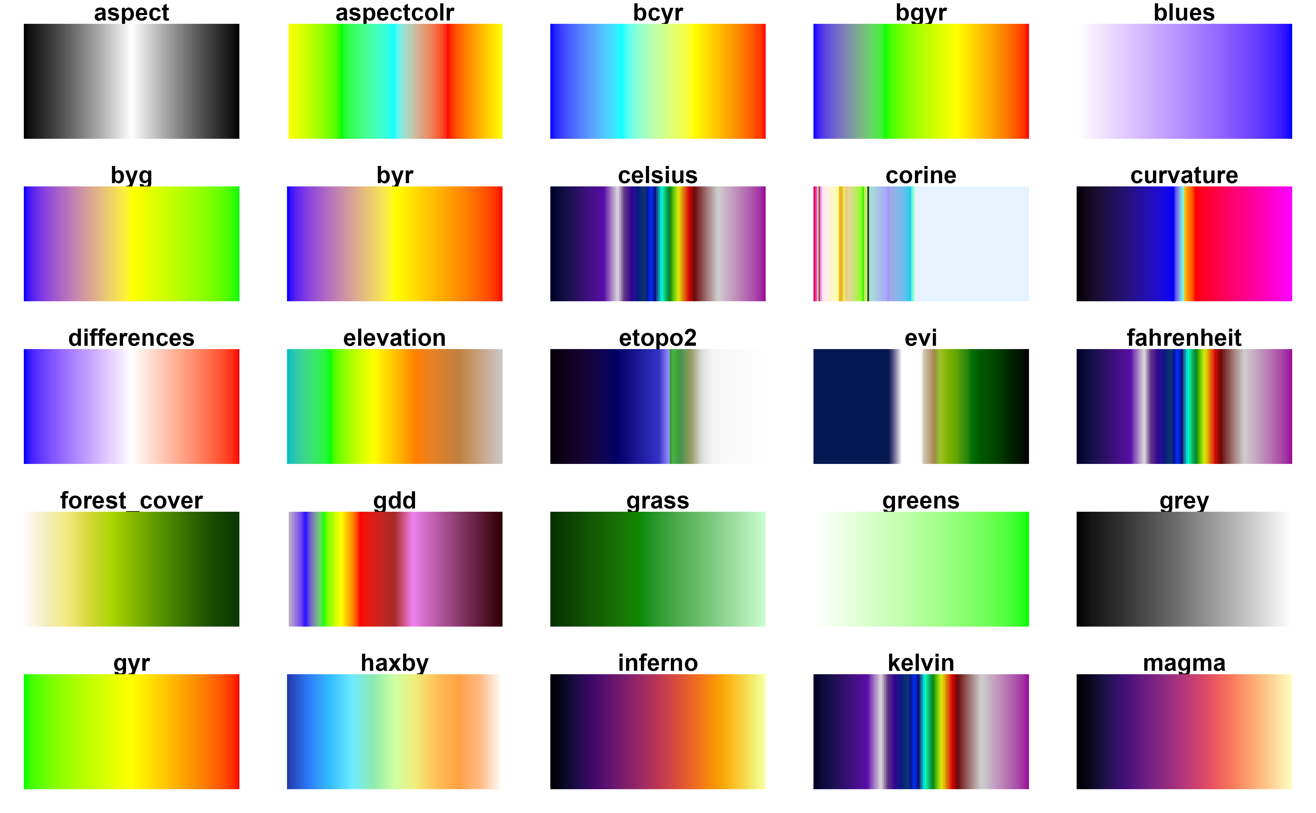
# Display all the GRASS palettes
data("grass_db")
pals_all <- unique(grass_db$pal)
# In batches
pals <- pals_all[c(1:25)]
# Helper function for plotting
ncols <- 128
rowcol <- grDevices::n2mfrow(length(pals))
opar <- par(no.readonly = TRUE)
par(mfrow = rowcol, mar = rep(1, 4))
for (i in pals) {
image(
x = seq(1, ncols), y = 1, z = as.matrix(seq(1, ncols)),
col = grass.colors(ncols, i), main = i,
ylab = "", xaxt = "n", yaxt = "n", bty = "n"
)
}
# }
# Display all the GRASS palettes
data("grass_db")
pals_all <- unique(grass_db$pal)
# In batches
pals <- pals_all[c(1:25)]
# Helper function for plotting
ncols <- 128
rowcol <- grDevices::n2mfrow(length(pals))
opar <- par(no.readonly = TRUE)
par(mfrow = rowcol, mar = rep(1, 4))
for (i in pals) {
image(
x = seq(1, ncols), y = 1, z = as.matrix(seq(1, ncols)),
col = grass.colors(ncols, i), main = i,
ylab = "", xaxt = "n", yaxt = "n", bty = "n"
)
}
 par(opar)
# Second batch
pals <- pals_all[-c(1:25)]
ncols <- 128
rowcol <- grDevices::n2mfrow(length(pals))
opar <- par(no.readonly = TRUE)
par(mfrow = rowcol, mar = rep(1, 4))
for (i in pals) {
image(
x = seq(1, ncols), y = 1, z = as.matrix(seq(1, ncols)),
col = grass.colors(ncols, i), main = i,
ylab = "", xaxt = "n", yaxt = "n", bty = "n"
)
}
par(opar)
par(opar)
# Second batch
pals <- pals_all[-c(1:25)]
ncols <- 128
rowcol <- grDevices::n2mfrow(length(pals))
opar <- par(no.readonly = TRUE)
par(mfrow = rowcol, mar = rep(1, 4))
for (i in pals) {
image(
x = seq(1, ncols), y = 1, z = as.matrix(seq(1, ncols)),
col = grass.colors(ncols, i), main = i,
ylab = "", xaxt = "n", yaxt = "n", bty = "n"
)
}
par(opar)