If you’ve ever worked with spatial data in R, this may ring a bell…
- Search for boundary data
- Figure out which version is “official”
- Download a shapefile
- Unzip it
- Load it
- Fix projections
- Repeat
While searching for new data sources, I found the excellent geoBoundaries database. However, accessing the data can be tedious since it’s provided as zipped shapefiles, and as any GIS professional knows, shapefiles should die!
Previously, the rgeoboundaries package was on CRAN and allowed to access the geoBoundaries API, but it was archived. So I decided to create my own version, and geobounds was born.
- Source code: https://github.com/dieghernan/geobounds
- pkgdown website: https://dieghernan.github.io/geobounds/
It connects directly to the excellent
geoBoundaries database and returns clean,
ready-to-use sf objects with a single function call. No manual downloads. No
shapefile messing.
This is how it works.
Installation
geobounds was recently accepted on CRAN, so just install it with:
install.packages("geobounds")
Load the package and other complementary packages:
library(geobounds)
library(sf)
library(ggplot2)
library(dplyr)
Getting administrative levels (ADM)
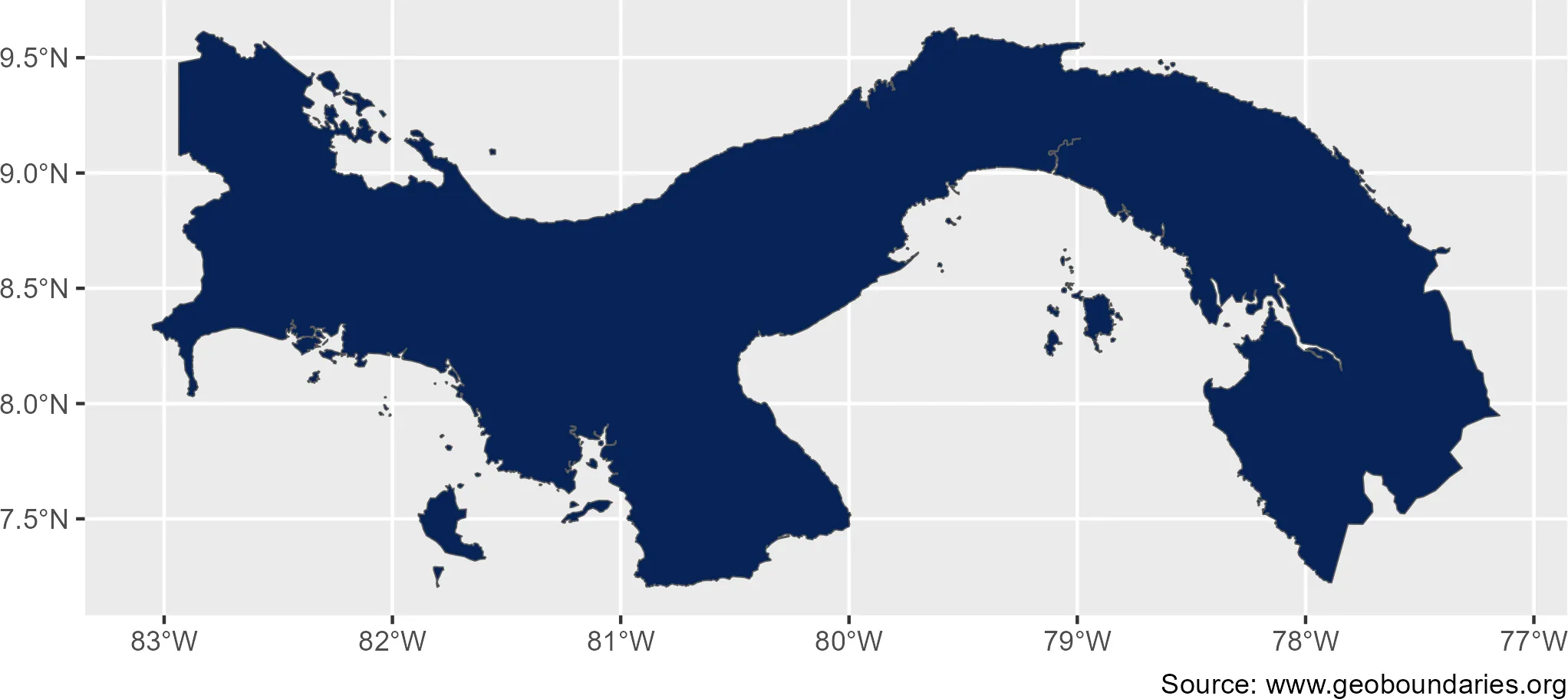
Administrative level 0 (ADM0) corresponds to countries:
# Panama

gb_get_adm0(country = "Panama") |>
  ggplot() +
  geom_sf(fill = "#072357") +
  labs(caption = "Source: www.geoboundaries.org")
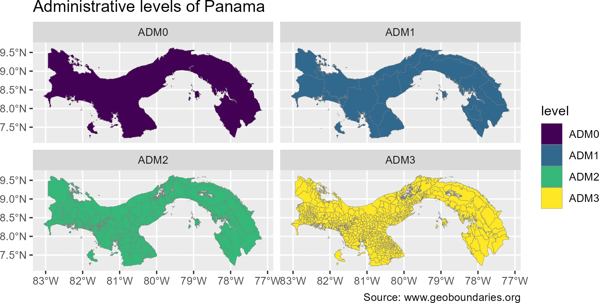
You can also retrieve multiple administrative levels at once. For example:
# Simplified files
gb_get(country = "Panama", adm_lvl = "all", simplified = TRUE) |>
  ggplot() +
  geom_sf(aes(fill = shapeType), color = "grey50", linewidth = 0.1) +
  facet_wrap(vars(shapeType)) +
  scale_fill_viridis_d() +
  labs(
    title = "Administrative levels of Panama",
    fill = "level",
    caption = "Source: www.geoboundaries.org"
  )
Global Composite Boundaries (CGAZ)
When you download individual country files, each country reflects its own view of borders. This results in:
- Overlapping boundaries
- Geographic gaps
- Disputed territories
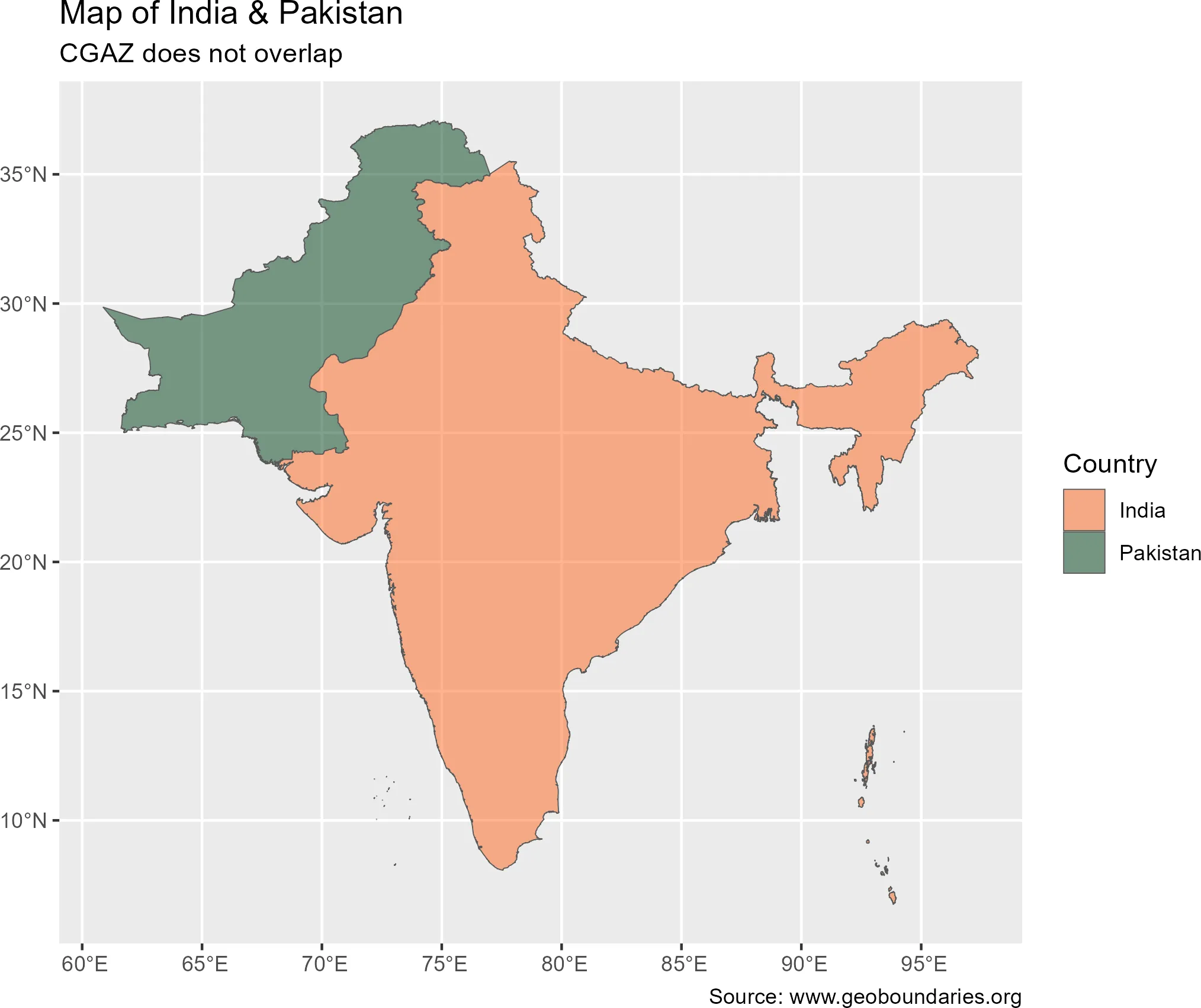
For clean global visualizations, geoBoundaries provides a Composite Global
Administrative Zones (CGAZ) dataset that can be accessed with gb_get_world().
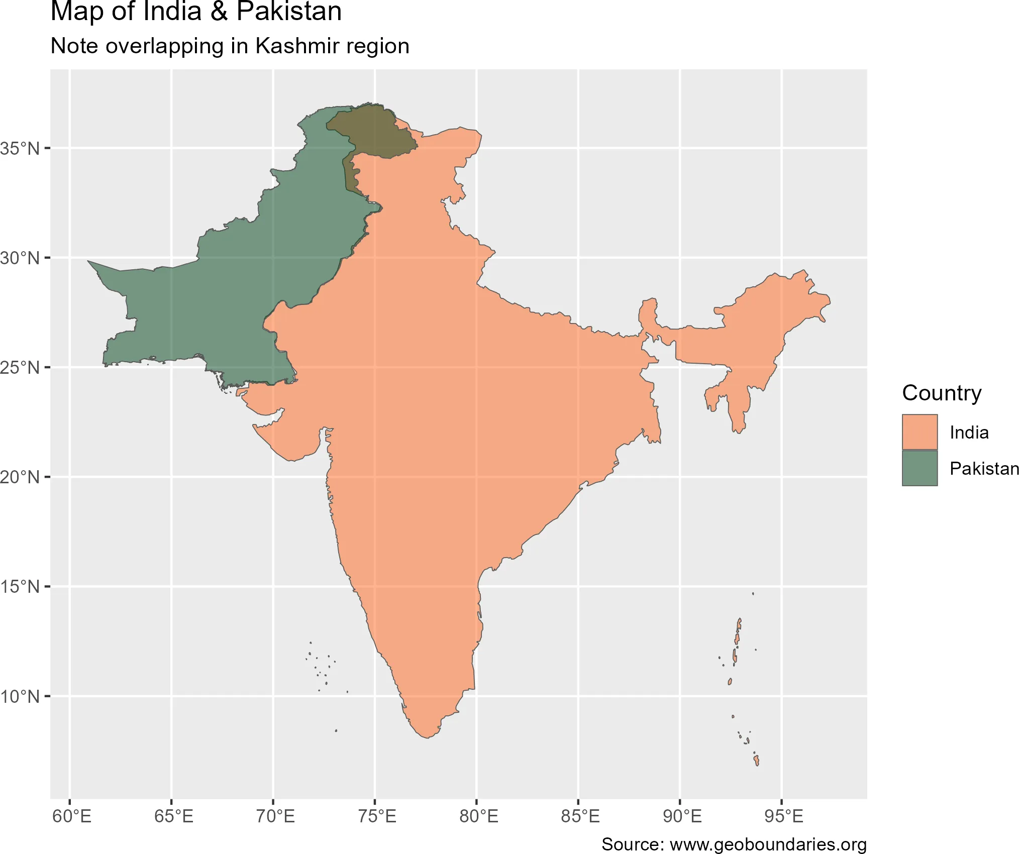
Here’s an example with country-level files:
# Using individual (gb_get_adm) shapefiles
gb_get_adm0(country = c("India", "Pakistan")) |>
  # Disputed area: Kashmir
  ggplot() +
  geom_sf(aes(fill = shapeName), alpha = 0.5) +
  scale_fill_manual(values = c("#FF671F", "#00401A")) +
  labs(
    fill = "Country",
    title = "Map of India & Pakistan",
    subtitle = "Note overlapping in Kashmir region",
    caption = "Source: www.geoboundaries.org"
  )
And here’s the same comparison using CGAZ with gb_get_world():
gb_get_world(c("India", "Pakistan")) |>
  ggplot() +
  geom_sf(aes(fill = shapeName), alpha = 0.5) +
  scale_fill_manual(values = c("#FF671F", "#00401A")) +
  labs(
    fill = "Country",
    title = "Map of India & Pakistan",
    subtitle = "CGAZ does not overlap",
    caption = "Source: www.geoboundaries.org"
  )
Understanding the data
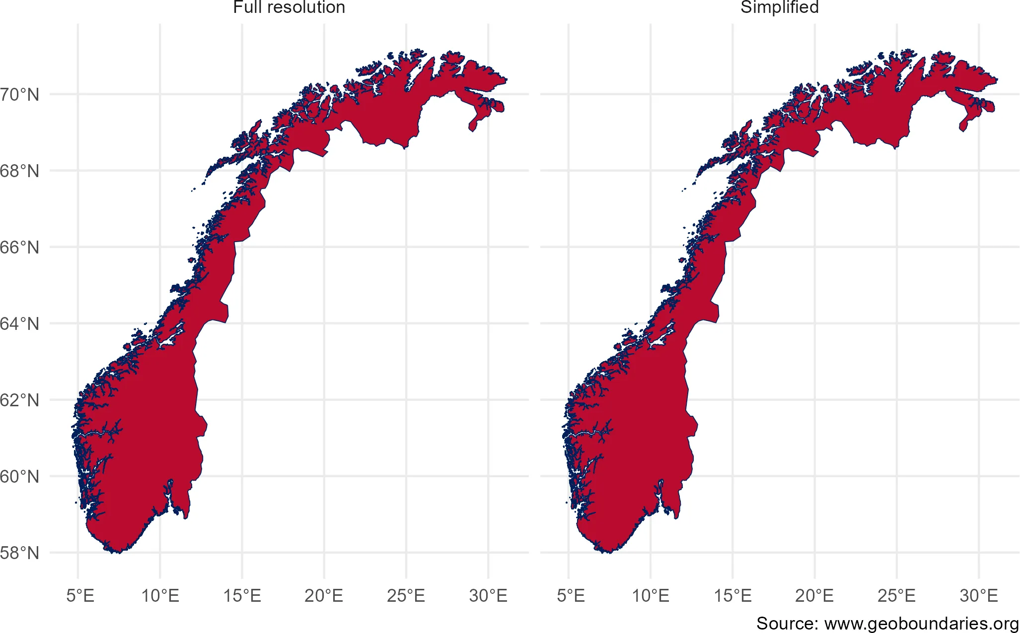
The geoBoundaries database undergoes rigorous quality assurance, including manual review and hand-digitization of physical maps. This ensures the highest level of spatial accuracy for scientific and academic research.
This precision comes at a cost: some files can be large and take longer to
download. For visualization and general mapping, we recommend using simplified
datasets by setting simplified = TRUE.
# Different resolutions
norway <- gb_get_adm0("NOR") |>
  mutate(res = "Full resolution")
print(object.size(norway), units = "Mb")
#> 26.5 Mb

norway_simp <- gb_get_adm0(country = "NOR", simplified = TRUE) |>
  mutate(res = "Simplified")
print(object.size(norway_simp), units = "Mb")
#> 1.5 Mb

norway_all <- bind_rows(norway, norway_simp)

# Plot ggplot2
ggplot(norway_all) +
  geom_sf(fill = "#BA0C2F", color = "#00205B") +
  facet_wrap(vars(res)) +
  theme_minimal() +
  labs(caption = "Source: www.geoboundaries.org")
Caching
Downloaded files are cached locally. That means:
- You download once
- Re-running your script is fast
- Your workflow stays reproducible
You can set the cache directory with:
gb_set_cache_dir("a/path/to/a/folder")
When should you use geobounds?
Use geobounds when:
- You need reliable global administrative boundaries
- You want reproducible workflows
- You prefer code over manual downloads
- You’re building maps, dashboards, or spatial analyses
Related Packages
geobounds is not alone in this space. Depending on your needs, you might also want to look at:
rnaturalearth
A very popular package to access Natural Earth datasets directly from R. It’s lightweight and great for quick global maps, especially at small scales.
If you need physical layers (rivers, coastlines, elevation) alongside political boundaries, this is often a good choice.
giscoR
If your focus is Europe, giscoR provides direct access to Eurostat GISCO data. It’s particularly useful for NUTS regions and European statistical boundaries.
osmdata
When administrative boundaries are not enough and you need OpenStreetMap features (roads, POIs, land use, etc.), osmdata gives you powerful querying capabilities.
Bottom line
I built geobounds to provide direct access to geoBoundaries products. I hope this package would help you in your GIS joruney.
Happy mapping!