Mapping Antarctica

Diego Hernangómez

Map projections with R
Issue 3 of 3

3 of 3

Issues

Creating maps with R is usually straightforward, but representations that cross the International Date Line or that use polar projections can be tricky.

Different spatial-data providers use different conventions: some break geometries at certain longitudes (for example, cutting the Chukchi Peninsula), while others omit portions of the data. These inconsistencies can produce awkward artifacts near the poles.

In this post, I fix the GISCO (European Commission) shapefile for Antarctica and produce clean orthographic maps.

# Libraries
library(tidyverse)
library(sf)
library(giscoR)
library(ggrepel)
library(rmapshaper)

# Define a common theme for the maps.
background <- "#E2ECF2"

map_family <- "inter-tight"
sysfonts::font_add_google("Inter Tight", family = map_family)
showtext::showtext_opts(dpi = knitr::opts_chunk$get("dpi"))
showtext::showtext_auto()

theme_set(
  theme_grey(paper = background) +
    theme(
      text = element_text(family = map_family),
      plot.title = element_text(face = "bold"),
      plot.margin = margin(10, 10, 10, 10)
    )
)

Fixing the geometry

First, we retrieve the Antarctic geometry from GISCO and transform it to an orthographic projection centered on the South Pole.

antarct <- gisco_get_countries(year = 2024, resolution = 1, country = "ATA") %>%
  select(NAME = NAME_ENGL) |>
  # Orthographic projection centered on the South Pole
  st_transform(crs = "+proj=ortho +lat_0=-90 +lon_0=0")

ggplot(antarct) +
  geom_sf(fill = "lightblue")

South Pole-centered map of Antarctica with a gap extending from the coast toward the pole, caused by a polygon artifact.

Updated November 14, 2026. The original post showed how to repair the geometry by editing vertices manually. This version uses a buffer.

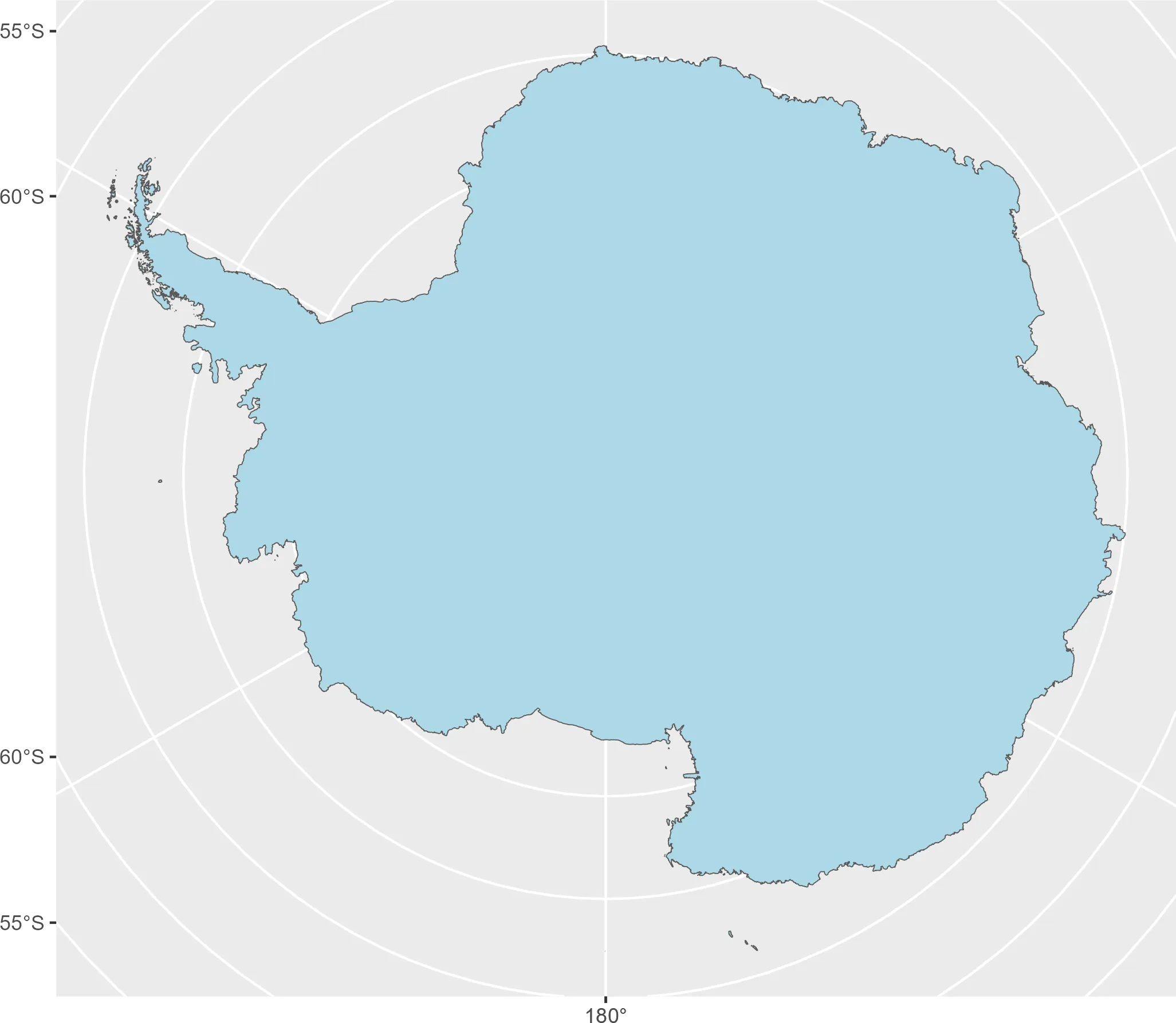
In the orthographic projection, a narrow gap runs inland from the coast. I close it by applying a 2-meter buffer:

# Regenerate initial shape
antarctica_fixed <- st_buffer(antarct, 2)

ggplot(antarctica_fixed) +
  geom_sf(fill = "lightblue")

South Pole-centered map of Antarctica after removing the polygon artifact. The landmass is continuous across the previously affected area.

Plotting examples

With the corrected geometry, we can draw the maps. Below are a few examples based on proposed Antarctic flag designs.

Graham Bartram’s proposal (1996)

A simple rendition of Bartram’s original concept:

bbox <- st_bbox(antarctica_fixed) # For limits on the panel

antarctica_fixed |>
  ggplot() +
  geom_sf(fill = "white", color = NA) +
  theme(
    panel.background = element_rect(fill = "#009fdc"),
    panel.grid = element_blank(),
    axis.text = element_blank(),
    axis.ticks = element_blank()
  ) +
  labs(title = "Graham Bartram's proposal") +
  coord_sf(
    xlim = c(bbox[c(1, 3)]) * 1.8,
    ylim = c(bbox[c(2, 4)]) * 1.4
  )

Antarctic flag design with a white silhouette of the continent on a blue background.

Emblem of the Antarctic Treaty

This example uses graticules to create a concentric “bullseye” pattern around Antarctica. Generating such graticules and merging meridians requires a few extra steps to avoid small gaps near the pole.

# Need graticules
grats <- giscoR::gisco_get_countries() |>
  st_transform(st_crs(antarctica_fixed)) |>
  # Specify the cuts of the graticules
  st_graticule(
    lat = c(-80, -70, -60),
    lon = seq(-180, 180, 30),
    ndiscr = 10000,
    margin = 0.000001
  )


ggplot(grats) +
  geom_sf(color = "darkblue")

Polar coordinate grid centered on the South Pole, with concentric latitude circles and radial longitude lines.

We merge meridians so the area around the South Pole is filled. st_graticule() can leave a tiny hole at the pole, and we fix this by joining complementary meridians.

# Merge meridians
merid <- lapply(seq(-180, 0, 30), function(x) {
  df <- grats |>
    filter(type == "E") |>
    filter(degree %in% c(x, x + 180))

  df2 <- df |>
    st_geometry() |>
    st_cast("MULTIPOINT") |>
    st_union() |>
    st_cast("LINESTRING")

  sf_x <- st_sf(
    degree = x,
    type = "E",
    geometry = df2
  )
}) |> bind_rows()


grats_end <- merid |>
  bind_rows(grats |>
    filter(type != "E"))

We then cut and color the resulting graticules so they form the emblem-like pattern.

# Cut since some grats should be colored differently

antarctica_simp <- rmapshaper::ms_simplify(antarctica_fixed, keep = 0.005)
grats_yes <- st_intersection(grats_end, antarctica_simp)
grats_no <- st_difference(grats_end, antarctica_simp)

antarctica_simp |>
  ggplot() +
  geom_sf(fill = "white", color = NA) +
  theme(
    panel.background = element_rect(fill = "#072b5f"),
    panel.grid = element_blank(),
    axis.text = element_blank(),
    axis.ticks = element_blank()
  ) +
  geom_sf(data = grats_yes, color = "#072b5f", linewidth = 1) +
  geom_sf(data = grats_no, color = "white", linewidth = 1) +
  coord_sf(
    xlim = c(bbox[c(1, 3)]) * 1.8,
    ylim = c(bbox[c(2, 4)]) * 1.4
  ) +
  labs(title = "Emblem of the Antarctic Treaty")

Antarctic Treaty emblem with a white Antarctic silhouette and polar coordinate grid on a dark blue background.

Bartram’s redesigned Antarctic flag

In 2024, Graham Bartram revealed a new version of his original flag as part of a global campaign to raise awareness about the growing problem of microplastic pollution. The new design keeps the familiar white outline of Antarctica but swaps the plain blue background for one filled with countless tiny, colorful dots. These dots represent the microscopic bits of plastic that have been discovered even in the planet’s most untouched places, including the Antarctic ice and its surrounding oceans.

Because the design relies on randomness, we approximate it using the following procedure:

Sample random points across the Antarctic polygon.
Build Voronoi polygons from those points, then apply a small negative buffer to create gaps.
Randomly sample the resulting polygons to increase visual noise.
Color polygons so larger areas remain white while smaller polygons use shades of pink and magenta.

# Use the repaired Antarctic geometry

set.seed(2024)
# Sample, Voronoi and negative buffer
plastics <- st_sample(antarctica_fixed, 3000) |>
  st_union() |>
  st_voronoi(envelope = st_geometry(antarctica_fixed)) |>
  st_collection_extract() |>
  st_buffer(dist = -10000)


# Keep only those properly included in the outline

toinc <- st_contains_properly(antarctica_fixed, plastics, sparse = FALSE) |>
  as.vector()

# Select random chunks
plastic_end <- plastics[toinc, ] |>
  st_as_sf() |>
  slice_sample(prop = 0.75)

ggplot(plastic_end) +
  geom_sf(fill = "darkblue")

Map of Antarctica filled with randomly distributed blue points inside the continent boundary.

# Random coloring

plastic_end$area <- st_area(plastic_end) |> as.double()

plastic_end$fill <- sample(c("#ff00ec", "#9e00ec"), nrow(plastic_end), replace = TRUE)
plastic_end$fill <- ifelse(plastic_end$area > quantile(plastic_end$area, probs = 0.4),
  "white",
  plastic_end$fill
)

bbox2 <- st_bbox(plastic_end)
ggplot() +
  geom_sf(data = plastic_end, aes(fill = fill), color = NA, linewidth = 0) +
  scale_fill_identity() +
  theme(
    panel.background = element_rect(fill = "#009fdc"),
    panel.grid = element_blank(),
    axis.text = element_blank(),
    axis.ticks = element_blank()
  ) +
  labs(title = "New redesign") +
  coord_sf(
    xlim = c(bbox2[c(1, 3)] * 1.8),
    ylim = c(bbox2[c(2, 4)]) * 1.4
  )

Antarctic flag variation with the continental silhouette formed by scattered white points on a blue background.

How to cite this post

For attribution, please cite this work as:

Hernangómez, D. (2025, October 25). Mapping Antarctica. One World. https://dieghernan.github.io/202510_mapping-antarctica/

BibTeX

   @misc{post20251025-mapping-antarctica,
  author = {Hernangómez, Diego},
  title = {Mapping Antarctica},
  year = {2025},
  month = oct,
  howpublished = {One World},
  url = {https://dieghernan.github.io/202510_mapping-antarctica/},
}
 