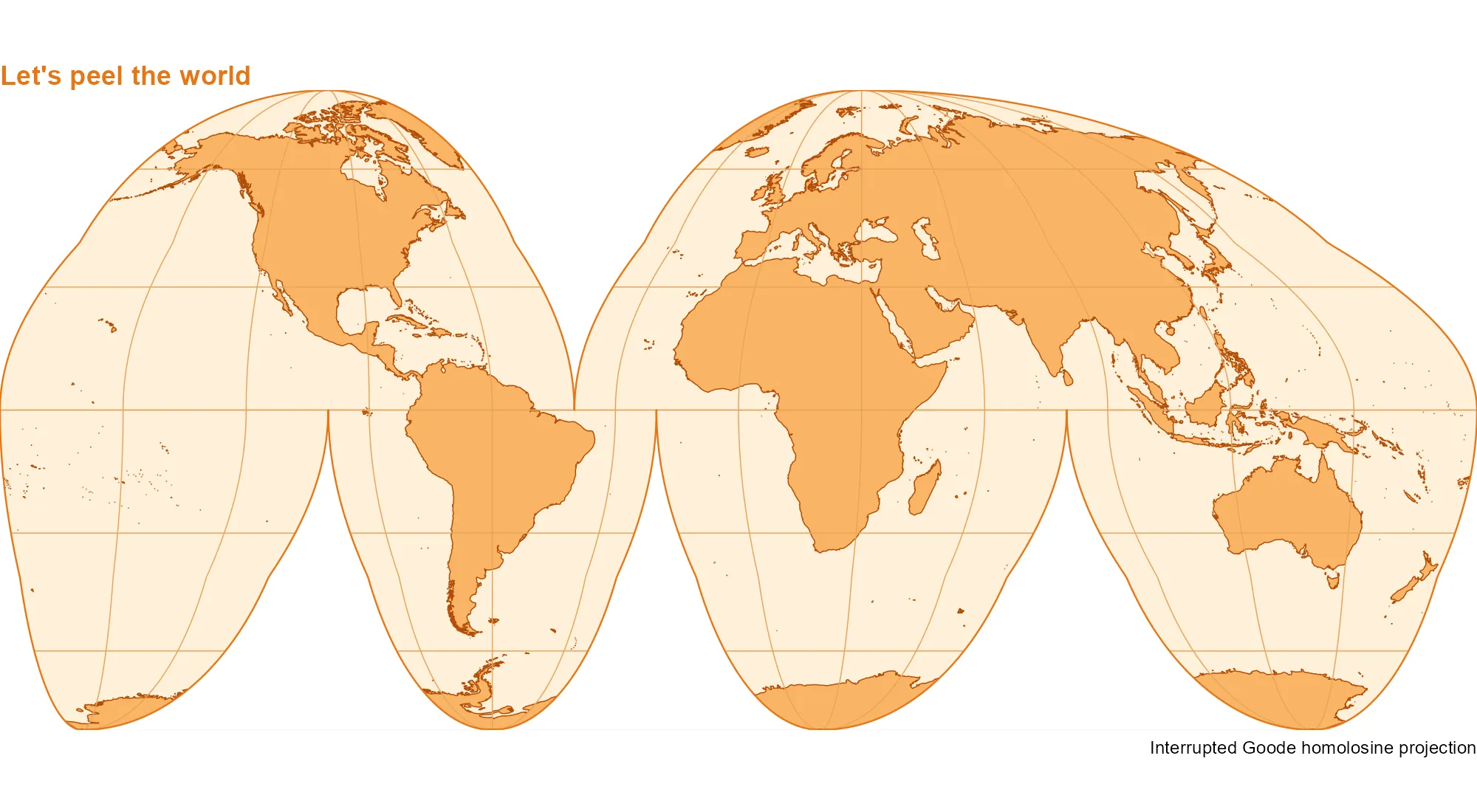
What would happen if we peeled the Earth like an orange? The interrupted Goode homolosine projection gives us something close to that! This equal-area projection preserves relative areas while splitting the world map into lobes. Add a few shades of orange and our world is ready to peel.
Let’s make it with sf, giscoR and ggplot2. First, we get the coastlines and draw the outline, following the cuts between the lobes.
library(sf)
library(ggplot2)
library(giscoR)

world <- gisco_get_coastal_lines(resolution = 10)
goode_crs <- "+proj=igh"
lat <- c(90:-90, rep(c(-90:0, 0:-90), 3), -90:90, 90:0, 0:90, 90)
lon <- c(
  rep(180, 181),
  rep(c(80.01, 79.99, -19.99, -20.01, -99.99, -100.01), each = 91),
  rep(-180, 181),
  rep(c(-40.01, -39.99), each = 91),
  180
)
outline <- st_sfc(st_polygon(list(cbind(lon, lat))), crs = 4326) |>
  st_transform(goode_crs)
rectangle <- st_as_sfc(st_bbox(outline) * 1.1)
mask <- st_difference(rectangle, outline)
Next, we draw the meridians and parallels within each lobe so that they do not connect across the cuts.
lobes <- list(
  c(-180, -40, 0, 90), c(-40, 180, 0, 90),
  c(-180, -100, -90, 0), c(-100, -20, -90, 0),
  c(-20, 80, -90, 0), c(80, 180, -90, 0)
)
lines <- lapply(lobes, function(b) {
  west <- b[1] + 0.01
  east <- b[2] - 0.01
  south <- max(b[3], -89.99)
  north <- min(b[4], 89.99)
  meridians <- seq(-180, 180, 30)
  meridians <- meridians[meridians > west & meridians < east]
  parallels <- seq(-60, 60, 30)
  parallels <- parallels[parallels >= south & parallels <= north]
  c(
    lapply(meridians, function(x) {
      st_linestring(cbind(x, seq(south, north, length.out = 181)))
    }),
    lapply(parallels, function(y) {
      st_linestring(cbind(seq(west, east, length.out = 361), y))
    })
  )
})
grat <- st_sfc(do.call(c, lines), crs = 4326) |>
  st_transform(goode_crs)
Finally, we add the orange palette. The mask hides anything outside the outline and keeps the edges of our peel tidy.
ggplot() +
  geom_sf(data = outline, fill = "#FFF0D9", colour = NA) +
  geom_sf(data = world, fill = "#F9B566", colour = "#B34D08", linewidth = 0.25) +
  geom_sf(data = grat, fill = NA, colour = "#E8A45B", linewidth = 0.25) +
  geom_sf(data = mask, fill = "white", colour = NA) +
  geom_sf(data = outline, fill = NA, colour = "#E87516", linewidth = 0.4) +
  coord_sf(
    crs = goode_crs,
    xlim = st_bbox(outline)[c("xmin", "xmax")],
    ylim = st_bbox(outline)[c("ymin", "ymax")],
    expand = FALSE,
    datum = NA
  ) +
  theme_void() +
  theme(
    plot.background = element_rect(fill = "white", colour = NA),
    plot.title = element_text(color = "#E87516", face = "bold")
  ) +
  labs(
    title = "Let's peel the world",
    caption = "Interrupted Goode homolosine projection"
  )
References
The outline and masking approach follows Claus O. Wilke’s Interrupted Goode homolosine example. For more on map projections, see Pyranhia’s Projections cartographiques : le guide pour ne pas y laisser sa santé mentale (in French).