I recently published my project Postal codes of Spain, with estimated postal areas, an interactive map and GeoPackage downloads. But there is something we have not looked at yet: how do those address points become polygons? The answer is… Voronoi polygons.
What is a Voronoi polygon?
Imagine a few shops on a flat map. Which one is closest to your house? Ask that question for every location and give each shop its own color. The result is a Voronoi diagram, also known as a Voronoi tessellation, Voronoi decomposition, Voronoi partition or Dirichlet tessellation. This technique divides a plane into regions based on the distance to a given set of points.
In our example, each shop is a site, or generating point. Its Voronoi cell, also called a Thiessen polygon, contains the locations at least as close to that site as to any other. Along a shared edge, two sites are equally close. Where several cells meet, there may be a tie between more sites. With ordinary straight-line distance, the edges follow perpendicular bisectors between sites. Some cells extend indefinitely, so maps usually show them clipped to a study area.
The name honors Georgy Voronoi, who studied these partitions in the early twentieth century. The idea has earlier roots, including Dirichlet’s nineteenth-century work (hence the name Dirichlet tessellation). Pokojski and Pokojska (2018) review the history and geographical applications.
These partitions are useful for exploring proximity to shops or public services, assigning areas to weather stations and studying spatial patterns. For example, Thiessen polygons can supply area weights when estimating rainfall from rain gauges. The underlying question is always about the chosen distance: the nearest hospital in a straight line may not be the quickest one to reach.
A tiny example in R
Let’s start with five points in an imaginary square, including one at its center, using just sf and ggplot2. The coordinates have arbitrary units and no geographical coordinate reference system.
library(sf)
library(ggplot2)

# Define a common theme for the maps.
background <- "#faf8f2"
ink <- "#203b47"

theme_set(
  theme_void() +
    theme(
      plot.background = element_rect(fill = background, colour = NA),
      panel.background = element_rect(fill = background, colour = NA),
      plot.title = element_text(face = "bold", colour = ink),
      plot.subtitle = element_text(colour = ink),
      plot.caption = element_text(colour = "grey40", hjust = 0),
      legend.position = "bottom",
      plot.margin = margin(10, 10, 10, 10)
    )
)

sites <- data.frame(
  site = c("A", "B", "C", "D", "E"),
  x = c(2, 7, 3, 8, 5),
  y = c(2, 3, 8, 7, 5)
)

toy_points <- st_as_sf(sites, coords = c("x", "y"))

study_area <- st_as_sfc(st_bbox(c(xmin = 0, ymin = 0, xmax = 10, ymax = 10)))

toy_cells <- toy_points |>
  st_union() |>
  st_voronoi(envelope = study_area) |>
  st_collection_extract("POLYGON") |>
  st_intersection(study_area)

ggplot() +
  geom_sf(
    data = toy_cells,
    fill = c("#a8dadc", "#f4c89a", "#c6b8df", "#bfd59b", "#f2b5c4"),
    colour = "white", linewidth = 1
  ) +
  geom_sf(data = toy_points, colour = "#203b47", size = 3) +
  geom_text(
    data = sites, aes(x, y, label = site),
    nudge_y = 0.5, colour = "#203b47", fontface = "bold"
  ) +
  coord_sf(datum = NA) +
  labs(
    title = "Five points, five Voronoi cells",
    subtitle = "Each location belongs to the closest site"
  )
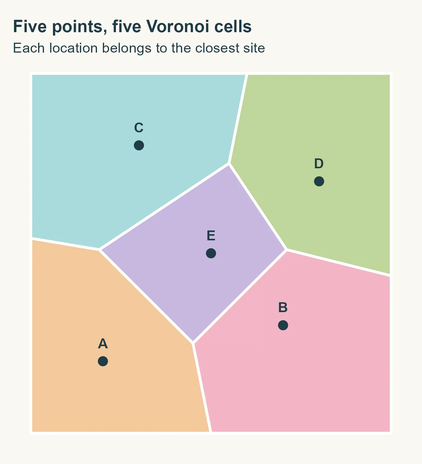
Five points, five cells. The point E at (5, 5) has a bounded cell
surrounded by the other four. The outer cells extend beyond the square and are
clipped to its edges. st_union() collects the points into one geometry,
st_voronoi() builds the diagram and st_intersection() clips it to our
square. The colors help us tell the cells apart. We have not assigned any postal
codes yet.
The diagram knows nothing about roads, rivers or administrative boundaries. As we move to postal points, we will need to make our choices about those boundaries explicit.
Before we start: what are we estimating?
The Spanish project uses CartoCiudad address points with their postal codes. It follows Goerlich (2022), who develops an idea presented by Sánchez (2020). The updated online version describes the method in detail.
For Slovenia, we will use GISCO’s postal points, retrieved with giscoR. There is an important difference here: a representative point for a code tells us much less than thousands of addresses with that code. Detailed addresses help the partition follow their distribution more closely, although proximity alone still cannot reproduce postal delivery decisions.
We have not established that Slovenian postal areas should follow municipal boundaries. Imposing those boundaries is a modeling choice for this exercise, inspired by the Spanish workflow, rather than a verified property of the Slovenian postal system.
This post explains the workflow. The polygons we create are not official postal boundaries, and this exercise does not validate the GISCO postal data.
Getting the data
First, let’s get the municipal boundaries and postal points. We use the 2024 release of both datasets.
library(giscoR)
library(sf)
library(dplyr)

municipalities <- gisco_get_lau(
  year = 2024, country = "SI", epsg = 3035
) |>
  select(GISCO_ID, LAU_NAME) |>
  st_make_valid()

raw_points <- gisco_get_postalcodes(
  year = 2024, country = "SI", epsg = 3035
)
We work in ETRS89 / LAEA Europe (EPSG:3035), a projected coordinate system with coordinates in meters. This makes the 200 m and 50 m margins used later meaningful. Voronoi uses Euclidean distances in this plane, rather than road distances. The projection does not preserve every distance exactly either.
Before we start drawing, what have we actually downloaded?
postal_points <- raw_points |>
  mutate(POSTCODE = trimws(as.character(POSTCODE))) |>
  filter(!is.na(POSTCODE), POSTCODE != "") |>
  select(POSTCODE)

code_counts <- postal_points |>
  st_drop_geometry() |>
  count(POSTCODE, name = "points_per_code")

knitr::kable(data.frame(
  Indicator = c(
    "Municipalities", "Downloaded points", "Points with a postal code",
    "Distinct postal codes", "Codes represented by one point"
  ),
  Value = c(
    nrow(municipalities), nrow(raw_points), nrow(postal_points),
    nrow(code_counts), sum(code_counts$points_per_code == 1)
  )
))
| Indicator | Value |
|---|---|
| Municipalities | 212 |
| Downloaded points | 557 |
| Points with a postal code | 557 |
| Distinct postal codes | 557 |
| Codes represented by one point | 557 |
These counts give us a first look at the file, but they are not a quality check. They do not establish whether every code is present or whether the coordinates are correct. With one point per code, we will be drawing areas around representatives rather than estimating them from individual addresses.
Two points at exactly the same coordinates cannot generate separate Voronoi cells. We sort by postal code and keep the first point at each location, as in the original workflow. This is a reproducible tie-breaking rule, not evidence that the retained code is correct. The counts below show how many records we remove and how many locations have conflicting codes.
postal_points <- postal_points |> arrange(POSTCODE)

conflicts <- postal_points |>
  group_by(geometry) |>
  summarise(codes = n_distinct(POSTCODE), .groups = "drop") |>
  filter(codes > 1)

duplicates <- duplicated(postal_points$geometry)

knitr::kable(data.frame(
  Indicator = c("Duplicate locations removed", "Locations with conflicting codes"),
  Value = c(sum(duplicates), nrow(conflicts))
))
| Indicator | Value |
|---|---|
| Duplicate locations removed | 79 |
| Locations with conflicting codes | 16 |
postal_points <- postal_points[!duplicates, ]
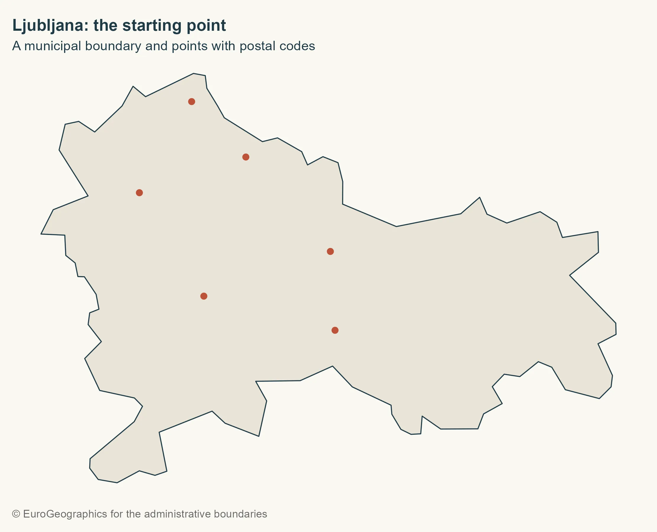
Starting with Ljubljana
Let’s pick Ljubljana and keep the points inside it. We use st_within() so that
a point exactly on a shared boundary is not assigned to both neighboring
municipalities.
city <- municipalities |> filter(LAU_NAME == "Ljubljana")

city_points <- st_filter(postal_points, city, .predicate = st_within)

base_map <- ggplot() +
  geom_sf(data = city, fill = "#e8e4d8", colour = ink, linewidth = 0.4)

gisco_attr <- gisco_attributions()

base_map +
  geom_sf(data = city_points, colour = "#bd5137", size = 2) +
  labs(
    title = "Ljubljana: the starting point",
    subtitle = "A municipal boundary and points with postal codes",
    caption = gisco_attr
  )
Building the cells
Each cell contains locations at least as close to its generating point as to any other point. Cell boundaries occur where distances to two points are equal. For this first demonstration, we keep all interior points, without the margins used in the national workflow.
cells <- city_points |>
  st_union() |>
  st_voronoi(envelope = st_as_sfc(st_bbox(city))) |>
  st_collection_extract("POLYGON") |>
  st_sf(geometry = _)

base_map +
  geom_sf(data = cells, fill = NA, colour = "#bd5137", linewidth = 0.5) +
  geom_sf(data = city_points, colour = ink, size = 2) +
  labs(
    title = "An area of proximity for every point",
    subtitle = "Cells still extend beyond the municipal boundary",
    caption = "Own elaboration using data from Eurostat / GISCO, 2024"
  )
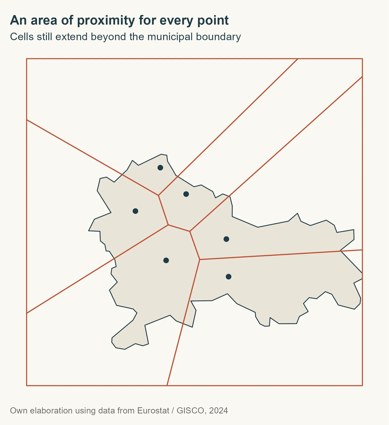
st_union() gathers the points so we build one diagram. One detail to keep in
mind: envelope supplies a working extent, but does not clip the cells to
the municipality. We need an intersection for that.
Clipping and recovering postal codes
It would be convenient if cells came out in the same order as the input points, but we should not rely on that. Instead, we recover each cell’s code with a spatial relationship before clipping. Each cell must contain exactly one generating point.
point_matches <- st_intersects(cells, city_points)

cells$POSTCODE <- city_points$POSTCODE[unlist(point_matches)]

clipped_geometry <- st_intersection(st_geometry(cells), st_geometry(city))

city_cells <- st_sf(
  POSTCODE = cells$POSTCODE[attr(clipped_geometry, "idx")[, 1]],
  geometry = clipped_geometry
)

city_areas <- city_cells |>
  group_by(POSTCODE) |>
  summarise(.groups = "drop") |>
  st_make_valid()

city_colours <- setNames(
  hcl.colors(nrow(city_areas), palette = "Dark 3"),
  sort(city_areas$POSTCODE)
)
city_labels <- st_sf(
  POSTCODE = city_areas$POSTCODE,
  geometry = st_point_on_surface(st_geometry(city_areas))
)

ggplot(city_areas) +
  geom_sf(aes(fill = POSTCODE), colour = background, linewidth = 0.6) +
  geom_sf(
    data = city_points, shape = 21, fill = ink,
    colour = background, size = 2.4
  ) +
  geom_sf_text(
    data = city_labels,
    aes(label = POSTCODE), colour = ink, fontface = "bold", size = 3.5
  ) +
  scale_fill_manual(values = city_colours, guide = "none") +
  coord_sf(datum = NA) +
  labs(
    title = "From points to estimated areas",
    subtitle = "Cells clipped and merged by postal code",
    caption = "Teaching example · Not official postal boundaries"
  )
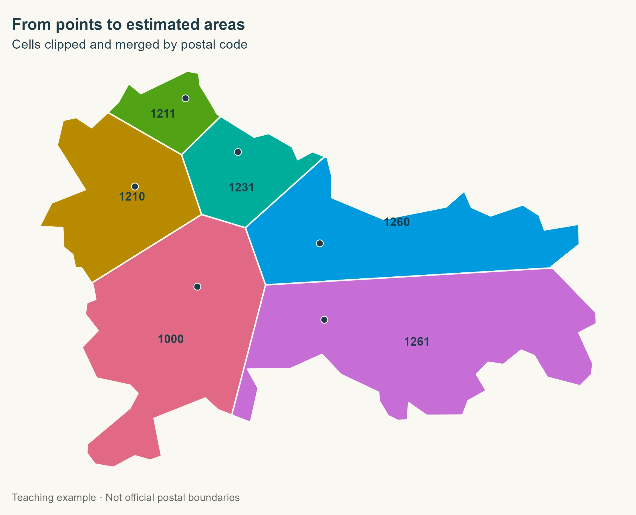
We intersect the geometry columns, then use the intersection’s idx matrix to
recover each cell’s postal code. This keeps the attribute assignment explicit.
Label positions are also calculated from geometries alone.
Grouping by postal code with summarise() merges the geometries. With many
addresses sharing a code, their cells would dissolve into one geometry, possibly
with several separate parts.
From one municipality to the whole country
Ljubljana is done. Now let’s repeat the operation for each component of each
municipality. Municipalities can have separate pieces: normalizing to
MULTIPOLYGON and then casting to POLYGON lets us handle them independently,
without automatically extending a code to a piece with no points.
The municipality ID and name apply to every component, so we mark those attributes as spatially constant before splitting the geometries.
components <- municipalities |>
  st_set_agr("constant") |>
  st_cast("MULTIPOLYGON") |>
  st_cast("POLYGON") |>
  mutate(component_id = row_number())
Why use an inward margin?
In the Spanish project, we first select addresses within an inward margin of 200 m. If none are found, we try 50 m. This reduces the influence of points close to a boundary, where small mismatches between layers may affect their assignment.
There is no universal rule behind these numbers. Goerlich describes a 20 m margin. The 200 m and 50 m choices come from my implementation. We keep them here to explain that workflow, although sparse postal points make it easier to exclude useful information. Comparing other margins would be a useful next step.
select_points <- function(component, postal_points) {
  for (margin in c(200, 50)) {
    interior <- st_buffer(st_geometry(component), -margin)

    if (all(st_is_empty(interior))) next

    selected_points <- st_filter(postal_points, interior,
      .predicate = st_within
    )

    if (nrow(selected_points) > 0) {
      return(selected_points)
    }
  }

  postal_points[0, ]
}
The margin only selects points: the resulting areas cover the original component, not the smaller buffered geometry. If both attempts fail, we leave the component unassigned. We do not borrow the nearest point from outside the municipality.
Three cases, one function
There are three cases to handle. With no points, we keep the component and
assign NA. If all selected points share a code, we assign it to the whole
component. We only need Voronoi when several codes are present: no need to split
an area that already has a single assignment.
build_areas <- function(component, postal_points) {
  selected_points <- select_points(component, postal_points)

  codes <- unique(selected_points$POSTCODE)

  if (length(codes) <= 1L) {
    component$POSTCODE <- if (length(codes)) codes else NA_character_
    return(component)
  }

  cells <- selected_points |>
    st_union() |>
    st_voronoi(envelope = st_as_sfc(st_bbox(component))) |>
    st_collection_extract("POLYGON") |>
    st_sf(geometry = _)

  point_matches <- st_intersects(cells, selected_points)

  cells$POSTCODE <- selected_points$POSTCODE[unlist(point_matches)]

  clipped_geometry <- st_intersection(
    st_geometry(cells),
    st_geometry(component)
  )

  result <- st_sf(
    POSTCODE = cells$POSTCODE[attr(clipped_geometry, "idx")[, 1]],
    geometry = clipped_geometry
  ) |>
    group_by(POSTCODE) |>
    summarise(.groups = "drop") |>
    st_make_valid()

  result$GISCO_ID <- component$GISCO_ID

  result$LAU_NAME <- component$LAU_NAME

  result$component_id <- component$component_id

  result
}

result <- lapply(seq_len(nrow(components)), function(i) {
  build_areas(components[i, ], postal_points)
}) |>
  bind_rows()
Handling unassigned areas
Can we fill any of the gaps? A component without points may belong to a municipality whose other components have information. We recover its code only if the municipality has one distinct recovered code. This is an imputation from the available data, not proof that the municipality really has just one code.
unique_codes <- result |>
  st_drop_geometry() |>
  filter(!is.na(POSTCODE)) |>
  distinct(GISCO_ID, POSTCODE) |>
  add_count(GISCO_ID) |>
  filter(n == 1)

unassigned_before <- sum(is.na(result$POSTCODE))

index <- match(result$GISCO_ID, unique_codes$GISCO_ID)

recoverable <- is.na(result$POSTCODE) & !is.na(index)

result$POSTCODE[recoverable] <- unique_codes$POSTCODE[index[recoverable]]
Before drawing the final map, let’s tidy up the geometries and keep only surfaces. Repairs can produce collections containing residual lines or points, which do not belong in an area layer. Dissolving by postal code also removes municipal boundaries between areas sharing that code.
keep_surfaces <- function(x) {
  geometry <- st_make_valid(st_geometry(x))

  geometry <- lapply(geometry, function(part) {
    if (!inherits(part, c("POLYGON", "MULTIPOLYGON", "GEOMETRYCOLLECTION"))) {
      return(st_multipolygon())
    }

    surfaces <- suppressWarnings(st_collection_extract(st_sfc(part), "POLYGON"))

    if (length(surfaces) == 0L || all(st_is_empty(surfaces))) {
      return(st_multipolygon())
    }

    st_cast(st_union(surfaces), "MULTIPOLYGON", warn = FALSE)[[1]]
  })

  st_geometry(x) <- st_sfc(geometry, crs = st_crs(x))

  x[!st_is_empty(x), ]
}

unassigned <- result |>
  filter(is.na(POSTCODE)) |>
  keep_surfaces()

postal_areas <- result |>
  filter(!is.na(POSTCODE)) |>
  group_by(POSTCODE) |>
  summarise(.groups = "drop") |>
  keep_surfaces() |>
  st_cast("MULTIPOLYGON")
The complete map
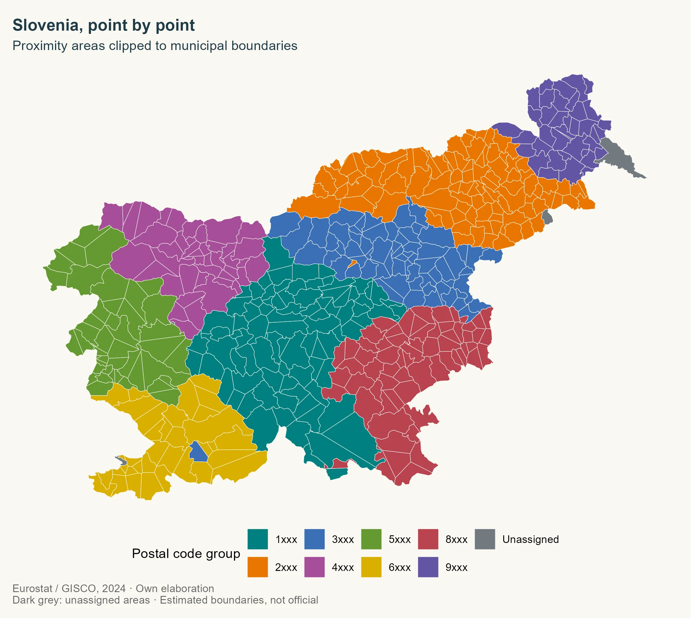
For the national overview, let’s color the areas by the first digit of their code. This keeps the map readable, without claiming that we have validated a classification of postal regions. Gray is reserved for unassigned components, with their own legend entry.
postal_colours <- c(
  "1" = "#007F7F", "2" = "#E87500", "3" = "#3B6FB6", "4" = "#A64E9A",
  "5" = "#649A32", "6" = "#D9AF00", "8" = "#B94350", "9" = "#6255A4",
  "Unassigned" = "#727A80"
)

postal_groups <- sort(unique(substr(postal_areas$POSTCODE, 1, 1)))

ggplot() +
  geom_sf(data = municipalities, fill = "#d5d2ca", colour = NA) +
  geom_sf(
    data = postal_areas,
    aes(fill = substr(POSTCODE, 1, 1)), colour = background, linewidth = 0.15
  ) +
  geom_sf(
    data = unassigned, aes(fill = "Unassigned"),
    colour = background, linewidth = 0.15
  ) +
  scale_fill_manual(
    values = postal_colours, name = "Postal code group",
    breaks = c(postal_groups, "Unassigned"),
    labels = c(paste0(postal_groups, "xxx"), "Unassigned")
  ) +
  coord_sf(datum = NA) +
  labs(
    title = "Slovenia, point by point",
    subtitle = "Proximity areas clipped to municipal boundaries",
    caption = paste("Eurostat / GISCO, 2024 · Own elaboration",
      "Dark grey: unassigned areas · Estimated boundaries, not official",
      sep = "\n"
    )
  )
Checking the result
The map is ready, but let’s check the geometry before going further. Are the polygons valid? Do assigned and unassigned areas cover the territory? Are there any appreciable overlaps? We allow one square meter for numerical differences in the geometry operations.
territory <- st_union(st_geometry(municipalities))

coverage <- st_union(c(st_geometry(postal_areas), st_geometry(unassigned)))

difference_m2 <- as.numeric(sum(st_area(st_sym_difference(territory, coverage))))

overlap_m2 <- as.numeric(
  sum(st_area(postal_areas)) + sum(st_area(unassigned)) - sum(st_area(coverage))
)

knitr::kable(data.frame(
  Indicator = c(
    "Codes with an estimated area", "Components assigned by municipal recovery",
    "Unassigned records", "Unassigned area (km²)",
    "Coverage difference (m²)", "Overlap (m²)"
  ),
  Value = round(c(
    nrow(postal_areas), sum(recoverable), nrow(unassigned),
    as.numeric(sum(st_area(unassigned))) / 1e6, difference_m2,
    overlap_m2
  ), 4)
))
| Indicator | Value |
|---|---|
| Codes with an estimated area | 468.0000 |
| Components assigned by municipal recovery | 4.0000 |
| Unassigned records | 6.0000 |
| Unassigned area (km²) | 150.2033 |
| Coverage difference (m²) | 0.0000 |
| Overlap (m²) | -0.0002 |
These checks verify the geometry, not postal accuracy. We could cover an entire country with valid polygons and still have a poor approximation of its delivery areas.
Back to Spain
We now have the full sequence: points, proximity areas, clipping and merging by postal code. The same steps work with much more detailed addresses, such as the CartoCiudad data in my Spanish postal codes project.
The input data matters as much as the algorithm. With one representative point per code, Voronoi mainly maps distances between representatives. With address points, it can better approximate where each code’s addresses are concentrated. It still knows nothing about delivery routes, physical barriers or official boundaries.
We have not compared these results with an independent postal source for Slovenia. Before using them for analysis, we would need to review coverage, coordinates, the relationship with municipalities and sensitivity to the margins. For now, we have a working example that shows how the polygons are built, one step at a time.
References
- Pokojski, W. & Pokojska, P. (2018). Voronoi diagrams – inventor, method, applications. Polish Cartographical Review, 50(3), 141–150. https://doi.org/10.2478/pcr-2018-0009.
- Goerlich, F. J. (2022). Elaboración de un mapa de códigos postales de España con recursos libres. Cómo evitar pagar por disponer de información de referencia. Working Papers Ivie, no. 2022-3. València: Ivie. https://doi.org/10.12842/WPIVIE_0322. Updated online version: https://www.uv.es/goerlich/Ivie/CodPost.html.
- Sánchez, J. I. (2020, November 13). “Así hice el mapa de los códigos postales de España con SIG y datos abiertos.” NoSoloSIG. https://www.nosolosig.com/articulos/asi-hice-el-mapa-de-los-codigos-postales-de-espana-con-sig-y-datos-abiertos.
- Hernangómez, D. (2026). Códigos postales de España [Dataset]. https://doi.org/10.5281/zenodo.23698418. https://dieghernan.github.io/codigospostales/.