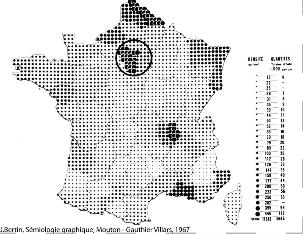
Recently the R Graph Gallery has incorporated a new post by Benjamin Nowak showing how to create a dot density map based on the work of the french cartographer Jacques Bertin (1918 - 2010):
In this post I would create a similar map for Iberia, and additionally I would show how to create a variation using a hexagonal grid instead of a rectangular one. This is the first issue of the series Beautiful Maps with R.
Libraries
I would use the following libraries for loading, manipulating and plotting spatial data (both raster and vector):
# Base spatial packages
library(terra)
library(sf)
# Spatial data
library(giscoR)
# Wrangling and plotting
library(tidyverse)
library(tidyterra)
library(ggtext)
# Additional for hex grids
# Supporting for units and bridge raster to polygon
library(units)
library(exactextractr)
Get the data
The first step is always to get the data we need. My final map would use as a base a circular layout with Iberia in the middle (that would be our observation window), so we can get the corresponding shapes and create a buffer around it.
After that, we would extract the population spatial distribution from GHSL - Global Human Settlement Layer. We would use the global file with a resolution of 1 km on Mollweide projection (ESRI:54009).
# Create observation window based the Iberian Peninsula and surroundings
# We create a buffered circle
owin <- gisco_get_countries(
  country = c("ES", "PT"),
  # We buffer in 3035 since I want my final map on this projection
  epsg = 3035,
  resolution = 60
) %>%
  st_geometry() %>%
  st_union() %>%
  st_centroid(of_largest_polygon = TRUE) %>%
  st_buffer(750000) %>%
  # But for extracting raster data we need this in Mollweide so far
  st_transform(crs = "ESRI:54009")

# Get additional shapes and cut them to the owin
regions <- gisco_get_nuts(resolution = 3, nuts_level = 2) %>%
  st_transform(st_crs(owin)) %>%
  st_intersection(owin)

countries <- gisco_get_countries(resolution = 3) %>%
  st_transform(st_crs(owin)) %>%
  st_intersection(owin)

# Base map
base_gg <- ggplot() +
  geom_sf(data = regions, fill = NA, color = "black", linewidth = 0.1) +
  geom_sf(data = countries, fill = NA, linewidth = 0.5, color = "black") +
  geom_sf(data = owin, fill = NA, linewidth = 0.75, color = "black")

base_gg
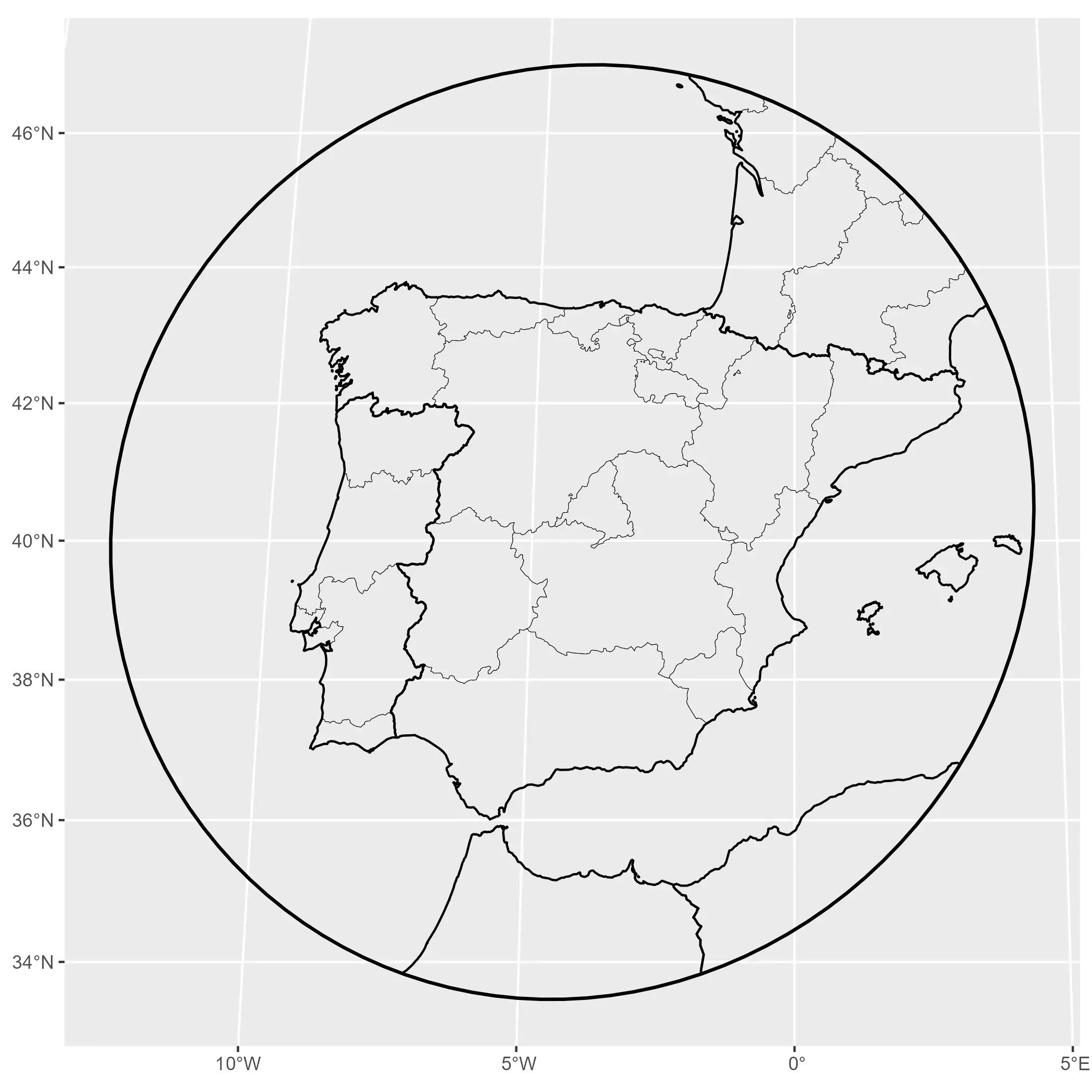
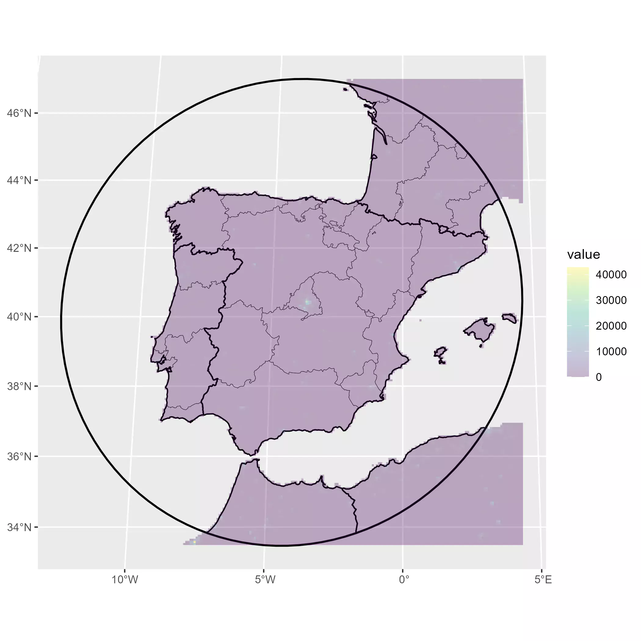
That would be our base map. Now we download programmatically the GHSL data and
we would check that everything is correct. At this point, it is interesting to
use the win argument when reading the raster with terra::rast(), as this
would allow us to load only the desired area with the subsequent improvement in
terms of performance.
# Download data
# We need the following file (download 305Mb)
url <- "https://jeodpp.jrc.ec.europa.eu/ftp/jrc-opendata/GHSL/GHS_POP_GLOBE_R2023A/GHS_POP_E2030_GLOBE_R2023A_54009_1000/V1-0/GHS_POP_E2030_GLOBE_R2023A_54009_1000_V1_0.zip"

# This is where I would store the file, you would need to modify the folder
fname <- file.path("~/R/mapslib/GHS", basename(url))
if (!file.exists(fname)) {
  download.file(url, fname)
}
zip_content <- unzip(fname, list = TRUE)
zip_content
#>                                                 Name    Length                Date
#> 1     GHS_POP_E2030_GLOBE_R2023A_54009_1000_V1_0.tif 263188307 2023-04-28 21:11:00
#> 2 GHS_POP_E2030_GLOBE_R2023A_54009_1000_V1_0.tif.ovr  88461532 2023-04-28 21:11:00
#> 3                         GHSL_Data_Package_2023.pdf   9761851 2023-10-27 14:30:00
#> 4           GHS_POP_GLOBE_R2023A_input_metadata.xlsx    137963 2023-04-30 10:42:00

# Unzip
unzip(fname, exdir = "~/R/mapslib/GHS", junkpaths = TRUE, overwrite = FALSE)

# Create the path to the file
global_tiff <- zip_content$Name[grepl("tif$", zip_content$Name)]
global_tiff_path <- file.path("~/R/mapslib/GHS", global_tiff)

# And read cropping to our owin
pop_init <- rast(global_tiff_path, win = as_spatvector(owin))

# Consistent naming of the layer
names(pop_init) <- "population"

ncell(pop_init)
#> [1] 2255923

# And check with tidyterra
base_gg +
  geom_spatraster(data = pop_init, maxcell = 50000) +
  scale_fill_viridis_c(na.value = "transparent", alpha = 0.3)
Data wrangling
The GHSL information contains the estimated population on each grid. However the file has a high resolution (more than 2 millions of cells) so for plotting purposes we are going to reduce (i.e. aggregate) the number of cells so we can have a better dot visualization. Once that we aggregate, we would compute the area of each new aggregated cell and compute the corresponding population density.
Instead of using the numeric range of densities, we would use categories for the final map, so we would classify the density into different groups:
# Reduce resolution for visualization
# Compute factor to reduce raster to (aprox) 100 rows:
nrow(pop_init)
#> [1] 1511
factor <- round(nrow(pop_init) / 100)

# Each new cell would contain the sum of population of the aggregated cells
pop_agg <- terra::aggregate(pop_init,
  fact = factor, fun = "sum",
  na.rm = TRUE
)


# Compute area of each new cell
pop_agg$area_km2 <- cellSize(pop_agg, unit = "km")

# Compute densities, mask to owin, convert to points and create categories
pop_points <- pop_agg %>%
  # Compute density by cell
  mutate(dens = population / area_km2) %>%
  select(dens) %>%
  # Mask to the countries shapes
  mask(as_spatvector(countries), touches = FALSE) %>%
  # SpatVector as points
  as.points() %>%
  # Categorize
  mutate(cat = case_when(
    dens < 25 ~ "A",
    dens < 50 ~ "B",
    dens < 100 ~ "C",
    dens < 250 ~ "D",
    dens < 500 ~ "E",
    dens < 1500 ~ "F",
    TRUE ~ "G"
  ))
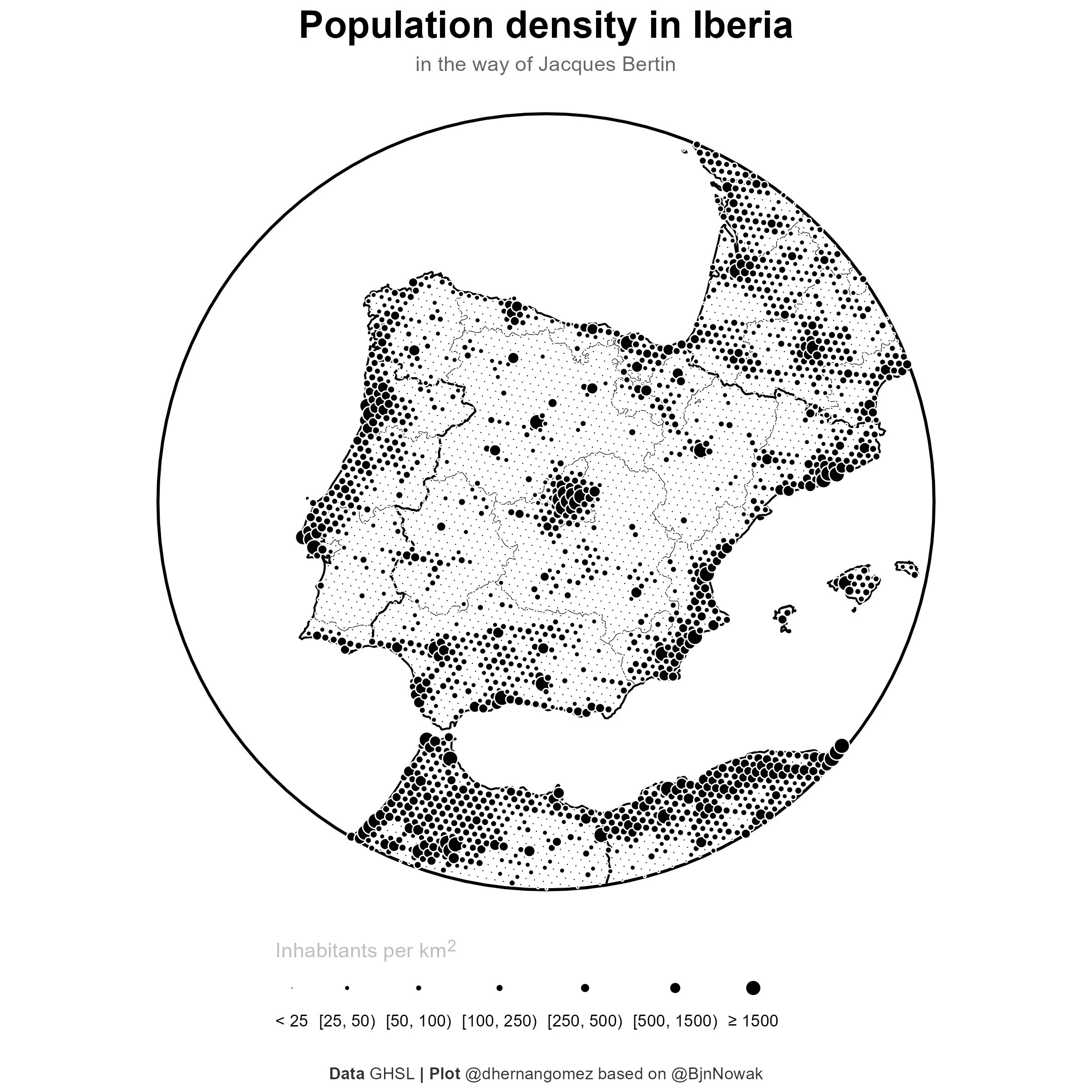
Final plot
And finally the map. In this case I would save it as a high resolution square map.
# Final plot
final_plot <- base_gg +
  # Layer, this object is a SpatVector instead of sf object
  geom_spatvector(
    pop_points,
    mapping = aes(size = cat),
    # Use a point with a border AND a fill
    pch = 21, color = "white", fill = "black", linewidth = 0.05
  ) +
  scale_size_manual(
    values = c(0.3, 1, 1.25, 1.5, 2, 2.5, 3.5),
    labels = c(
      "< 25", "[25, 50)", "[50, 100)", "[100, 250)",
      "[250, 500)", "[500, 1500)", "≥ 1500"
    ),
    guide = guide_legend(
      nrow = 1,
      title.position = "top",
      keywidth = 1,
      label.position = "bottom"
    )
  ) +
  labs(
    title = "**Population density in Iberia**",
    subtitle = "in the way of Jacques Bertin",
    size = "<span style='color:grey'>Inhabitants per km<sup>2</sup></span>",
    caption = "**Data** GHSL **| Plot** @dhernangomez based on @BjnNowak"
  ) +
  theme_void() +
  # This CRS for representation only
  coord_sf(expand = TRUE, crs = 3035) +
  theme(
    # plot.margin = margin(20,0,20,0,"cm"),
    plot.background = element_rect(fill = "white", color = NA),
    legend.position = "bottom",
    legend.margin = margin(r = 20, unit = "pt"),
    legend.title = element_markdown(),
    legend.key.width = unit(50, "pt"),
    plot.title = element_markdown(hjust = 0.5, size = 20),
    plot.subtitle = element_text(hjust = 0.5, color = "grey40"),
    plot.caption = element_markdown(
      color = "grey20",
      margin = margin(t = 20, b = 5, unit = "pt"),
      hjust = .5
    )
  )


ggsave("202312_finalmap.png", dpi = 300, width = 8, height = 8)

Alternative hexagonal grid
The previous plot is based on the centroids of each cell of the raster, that is, by definition, a rectangular grid. I would like also to experiment with hexagonal grids (i.e. grid of hexagons) since I have the feeling that looks more “natural” than the rectangular ones, that presents a regularity hardly seen in the wild.
The issue here is that terra does not produce this type of grids, however it
is possible to create them with sf::st_make_grid(), so the workflow for this
altenative is:
- Create a hexagonal grid, where each hexagon represents a similar area than each cell on the aggregated raster.
- Extract the values of the raster to the new grid.
- Finally, follow the same steps on data wrangling and plotting.
When working with sf::st_make_grid(square = FALSE), the parameter cellsize
should be the “diameter” of the hexagon instead of the area. Luckly, we can
infer this value since the area of a hexagon is
So we can extract \(d\) from the previous expression knowing the area \(A\) of the aggregated cells:
# Hex grid with sf ----

# Avg size of the cells on the aggregated grid
target_area <- cellSize(pop_agg, unit = "km") %>%
  pull() %>%
  mean() %>%
  as_units("km^2")

target_area
#> 224.7461 [km^2]

# Infer diam hex
diam_hex <- sqrt(2 * target_area / sqrt(3))
# Create hexagonal grid
pop_agg_sf <- st_make_grid(owin, cellsize = diam_hex, square = FALSE)

length(pop_agg_sf)
#> [1] 10340
ncell(pop_agg)
#> [1] 10100

area_km2 <- st_area(pop_agg_sf) %>%
  set_units("km^2") %>%
  as.double()

pop_agg_sf <- st_sf(area_km2 = area_km2, geom = pop_agg_sf)
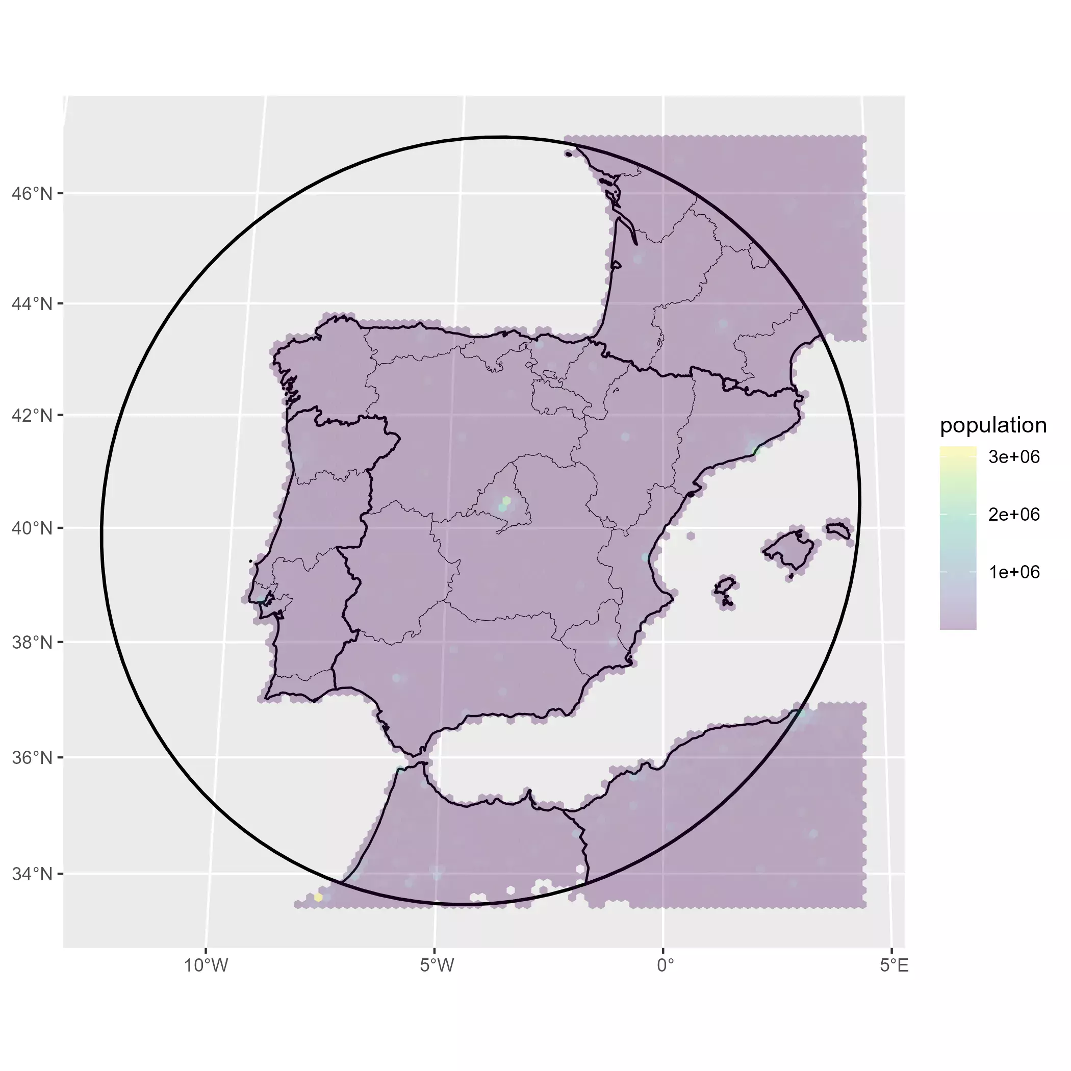
Now, we use exact_extract() to extract the population on each hexagonal grid.
# Extract aggregated population by hex cell
pop_agg_sf$population <- exact_extract(pop_init,
  y = pop_agg_sf,
  progress = FALSE,
  fun = "sum"
)


base_gg +
  geom_sf(
    data = pop_agg_sf %>% filter(population > 0),
    aes(fill = population), color = NA
  ) +
  scale_fill_viridis_c(na.value = "transparent", alpha = 0.3)
Finally we just compute densities, create categories and finally the map:
# Mask and categorize
pop_sf_points <- pop_agg_sf %>%
  # Compute density by cell
  mutate(dens = population / area_km2) %>%
  select(dens) %>%
  # To points and filter to country shape
  st_centroid(of_largest_polygon = TRUE) %>%
  st_filter(countries) %>%
  # Categorize
  mutate(cat = case_when(
    dens < 25 ~ "A",
    dens < 50 ~ "B",
    dens < 100 ~ "C",
    dens < 250 ~ "D",
    dens < 500 ~ "E",
    dens < 1500 ~ "F",
    TRUE ~ "G"
  ))

# Final plot
final_plot_hex <- base_gg +
  # Layer, this object is a sf object
  geom_sf(
    pop_sf_points,
    mapping = aes(size = cat),
    # Use a point with a border AND a fill
    pch = 21, color = "white", fill = "black", linewidth = 0.05
  ) +
  scale_size_manual(
    values = c(0.3, 1, 1.25, 1.5, 2, 2.5, 3.5),
    labels = c(
      "< 25", "[25, 50)", "[50, 100)", "[100, 250)",
      "[250, 500)", "[500, 1500)", "≥ 1500"
    ),
    guide = guide_legend(
      nrow = 1,
      title.position = "top",
      keywidth = 1,
      label.position = "bottom"
    )
  ) +
  labs(
    title = "**Population density in Iberia**",
    subtitle = "in the way of Jacques Bertin",
    size = "<span style='color:grey'>Inhabitants per km<sup>2</sup></span>",
    caption = "**Data** GHSL **| Plot** @dhernangomez based on @BjnNowak"
  ) +
  theme_void() +
  # This CRS for representation only
  coord_sf(expand = TRUE, crs = 3035) +
  theme(
    # plot.margin = margin(20,0,20,0,"cm"),
    plot.background = element_rect(fill = "white", color = NA),
    legend.position = "bottom",
    legend.margin = margin(r = 20, unit = "pt"),
    legend.title = element_markdown(),
    legend.key.width = unit(50, "pt"),
    plot.title = element_markdown(hjust = 0.5, size = 20),
    plot.subtitle = element_text(hjust = 0.5, color = "grey40"),
    plot.caption = element_markdown(
      color = "grey20",
      margin = margin(t = 20, b = 5, unit = "pt"),
      hjust = .5
    )
  )

ggsave("202312_finalmap_hex.png", dpi = 300, width = 8, height = 8)
And that’s it! Which one do you like the most? Let me know in the comments.
References
- Bertin J (1967). Sémiologie graphique. Les diagrammes. Les réseaux. Les cartes. Gauthier-Villars, Paris.
- European Commission. Joint Research Centre. (2023). GHSL data package 2023.. Publications Office, LU https://doi.org/10.2760/098587
- Hernangómez D (2023). “Using the tidyverse with terra objects: the tidyterra package Journal of Open Source Software, 8(91), 5751. ISSN 2475-9066 https://doi.org/10.21105/joss.05751
- Pesaresi M, Politis P (2023). “GHS-BUILT-C R2023A - GHS Settlement Characteristics, derived from Sentinel2 composite (2018) and other GHS R2023A data.” https://doi.org/10.2905/3C60DDF6-0586-4190-854B-F6AA0EDC2A30