Star Map with R | One world

A couple of weeks ago I was doing my daily check on StackOverflow when I found a question by Benjamin Smith that blew my mind: Creating Star Map Visualizations Based on Location and Date !!

Oh my! Can we do this with R? Answer is: Of course! In fact, Kim Fitter already worked on this two years ago, see his Celestial Maps. So I decided to put some work on this.

Since then, I also learnt that Benjamin and myself have been working on parallel on the same topic. He is preparing a R package named starBliss and hopefully this post would be of some help.

I have very little knowledge on this topic, so if you find errors or have any suggestions please let me know in the Comments section below

First things first: The data

The initial data source of all these projects (Kim, Benjamin and myself) is the same, and it is provided on the D3 plugin d3-celestial by Olaf Frohn. As Kim Fitter pointed out on his post, these data files present the problem (experienced by almost any sf user) of lines crossing the international date line (longitude 180º). I also found that some files are not valid as per sf::st_make_valid().

Solution? I processed and fixed almost every file (some of them as the corresponding to the Milky Way or the lines for Chinese constellations manually) to provide a set of files. That is the origin of my project Celestial Data, that provides all these files on several spatial formats. Please check out the repo to know more about it.

Creating a Star Map with R

The first step is loading a bunch of libraries that would help us on this cosmic task:

# Spatial manipulation
library(sf)
library(s2)
library(nominatimlite)

## Wrange data and dates
library(dplyr)
library(lubridate)
library(lutz)

## Visualization
library(ggplot2)
library(ggfx)
library(ggshadow)

Helper funs

Now we prepare some helper functions:

load_celestial() just downloads the corresponding .geojson from the Celestial Data repo¹ to a specific directory cachedir and loads it with sf::st_read().
pretty_lonlat() is a labeller that returns a decimal longitude or latitude coordinate in the format degrees/minutes/seconds (e.g a latitude 34.72782 would be converted into 34° 43’ 40.15” N).

Show load_celestial and pretty_lonlat()

load_celestial <- function(filename,
                           url = "https://cdn.jsdelivr.net/gh/dieghernan/celestial_data@main/data/",
                           cachedir = tempdir()) {
  if (!dir.exists(cachedir)) {
    stop(
      "Please create ",
      path.expand(cachedir),
      " directory",
      "first"
    )
  }

  url <- file.path(url, filename)
  local_path <- file.path(cachedir, filename)


  if (!file.exists(local_path)) {
    download.file(url, local_path, mode = "wb", quiet = TRUE)
  }

  celestial <- sf::st_read(local_path, quiet = TRUE)

  return(celestial)
}

pretty_lonlat <- function(x, type, accuracy = 2) {
  positive <- x >= 0

  # Decompose
  x <- abs(x)
  D <- as.integer(x)
  m <- (x - D) * 60
  M <- as.integer(m)
  S <- round((m - M) * 60, accuracy)

  # Get label
  if (type == "lon") {
    lab <- ifelse(positive > 0, "E", "W")
  } else {
    lab <- ifelse(positive > 0, "N", "S")
  }


  # Compose
  label <- paste0(D, "\u00b0 ", M, "' ", S, '\" ', lab)
  return(label)
}

Additionally, you may notice that on this d3-celestial demo there is some degree of rotation depending on the location and the time. I found how this is done on the d3-celestial plugin and I found the function getMST(dt, lng), that I ported to R (get_mst()). As per some of the research that I did this function computes the Mean Sidereal Time (MST) given a specific longitude (maybe then is more accurate Local Sidereal Time? Just wondering) expressed in degrees, following the formulas provided by Meeus (1998). If you want to know more on this I recommend this post by James Still.

So basically the input is a POSIXct date time and a given longitude and the result is an alternative longitude that we would use to adjust the projection of our Star Map. This would provide the rotation observed on d3-celestial plugin.

Show get_mst()

# Derive rotation degrees of the projection given a date and a longitude
get_mst <- function(dt, lng) {
  desired_date_utc <- lubridate::with_tz(dt, "UTC")


  yr <- lubridate::year(desired_date_utc)
  mo <- lubridate::month(desired_date_utc)
  dy <- lubridate::day(desired_date_utc)
  h <- lubridate::hour(desired_date_utc)
  m <- lubridate::minute(desired_date_utc)
  s <- lubridate::second(desired_date_utc)

  if ((mo == 1) || (mo == 2)) {
    yr <- yr - 1
    mo <- mo + 12
  }

  # Adjust times before Gregorian Calendar
  # See https://squarewidget.com/julian-day/
  if (lubridate::as_date(dt) > as.Date("1582-10-14")) {
    a <- floor(yr / 100)
    b <- 2 - a + floor(a / 4)
  } else {
    b <- 0
  }
  c <- floor(365.25 * yr)
  d <- floor(30.6001 * (mo + 1))

  # days since J2000.0
  jd <- b + c + d - 730550.5 + dy + (h + m / 60 + s / 3600) / 24
  jt <- jd / 36525

  # Rotation
  mst <- 280.46061837 + 360.98564736629 * jd +
    0.000387933 * jt^2 - jt^3 / 38710000.0 + lng

  # Modulo 360 degrees
  mst <- mst %% 360

  return(mst)
}

The final result would have an spherical outline. That means that we would need to perform an spherical cut. Did you know that in r-spatial the Earth is no longer flat? Thanks to s2 we can overcome this issue. Additionally, we would get rid of artifacts derived from the changes on the projection. This also includes some refinements to avoid empty/non-valid geometries as well as GEOMETRYCOLLECTION handling. The function sf_spherical_cut() would do that for us.

Show sf_spherical_cut()

# Cut a sf object with a buffer using spherical s2 geoms
# Optionally, project and flip

sf_spherical_cut <- function(x, the_buff, the_crs = sf::st_crs(x), flip = NULL) {
  # Get geometry type
  geomtype <- unique(gsub("MULTI", "", sf::st_geometry_type(x)))[1]

  # Keep the data frame, s2 drops it
  the_df <- sf::st_drop_geometry(x)
  the_geom <- sf::st_geometry(x)
  # Convert to s2 if needed
  if (!inherits(the_buff, "s2_geography")) {
    the_buff <- sf::st_as_s2(the_buff)
  }

  the_cut <- the_geom %>%
    # Cut with s2
    sf::st_as_s2() %>%
    s2::s2_intersection(the_buff) %>%
    # Back to sf and add the df
    sf::st_as_sfc() %>%
    sf::st_sf(the_df, geometry = .) %>%
    dplyr::filter(!sf::st_is_empty(.)) %>%
    sf::st_transform(crs = the_crs)

  # If it is not POINT filter by valid and non-empty
  # This if for performance
  if (!geomtype == "POINT") {
    # If any is GEOMETRYCOLLECTION extract the right value
    if (any(sf::st_geometry_type(the_cut) == "GEOMETRYCOLLECTION")) {
      the_cut <- the_cut %>%
        sf::st_collection_extract(type = geomtype, warn = FALSE)
    }

    the_cut <- the_cut %>%
      dplyr::filter(!is.na(sf::st_is_valid(.)))
  }

  if (!is.null(flip)) {
    the_cut <- the_cut %>%
      dplyr::mutate(geometry = geometry * flip) %>%
      sf::st_set_crs(the_crs)
  }

  return(the_cut)
}

Inputs

Now we are ready to start creating our visualization. We need only two inputs:

A desired location, that we would geocode with nominatimlite.
A specific moment of time.

# Inputs
desired_place <- "Madrid, Spain"

# We are not using yet the timezone
desired_date <- make_datetime(
  year = 2015,
  month = 9,
  day = 22,
  hour = 3,
  min = 45
)

# Geocode place with nominatimlite
desired_place_geo <- geo_lite(desired_place, full_results = TRUE)

desired_place_geo %>%
  select(address, lat, lon)
#> # A tibble: 1 × 3
#>   address                                                                                    lat   lon
#>   <chr>                                                                                    <dbl> <dbl>
#> 1 Madrid, Área metropolitana de Madrid y Corredor del Henares, Comunidad de Madrid, España  40.4 -3.70

# And get the coordinates
desired_loc <- desired_place_geo %>%
  select(lat, lon) %>%
  unlist()

desired_loc
#>       lat       lon 
#> 40.416705 -3.703582

With respect to our object desired_date, it is quite relevant for accurate plotting to specify the correct time zone. Since we already now the latitude and longitude of our desired location, we can easily get that with the lutz package:

desired_date
#> [1] "2015-09-22 03:45:00 UTC"

# Get tz
get_tz <- tz_lookup_coords(desired_loc[1], desired_loc[2], warn = FALSE)

get_tz
#> [1] "Europe/Madrid"

# Force it to be local time
desired_date_tz <- force_tz(desired_date, get_tz)

desired_date_tz
#> [1] "2015-09-22 03:45:00 CEST"

About time zones

Some online shops that creates this kind of maps (I won’t post links) includes this script:

... 

'selectedHour': '22',
'selectedMinute': '00',

...

This means that those shops are really creating the map at YYYY-MM-DD 22:00:00 UTC. If you want to exactly replicate that (even though that night sky is not accurate, think that in New Zealand the local time at that moment would be 10:00 hence no stars are visible) you would need to adjust desired_date_tz as:

as_datetime(paste(as.Date(desired_date_tz), "22:00:00"), tz = "UTC")
#> [1] "2015-09-22 22:00:00 UTC"

# That would really correspond to 10:00
as_datetime(paste(as.Date(desired_date_tz), "22:00:00"), tz = "UTC") %>%
  with_tz("Pacific/Auckland")
#> [1] "2015-09-23 10:00:00 NZST"

Setup

Now we can start creating our buffers and projections, that would help us to crop the celestial data objects.

I noticed also that the location demo of d3-celestial.js uses Airy projection, so we are going to replicate that as well:

# Get the rotation and prepare buffer and projection

# Get right degrees
lon_prj <- get_mst(desired_date_tz, desired_loc[2])
lat_prj <- desired_loc[1]

c(lon_prj, lat_prj)
#>      lon      lat 
#> 23.15892 40.41670

# Create proj4string w/ Airy projection

target_crs <- paste0("+proj=airy +x_0=0 +y_0=0 +lon_0=", lon_prj, " +lat_0=", lat_prj)


target_crs
#> [1] "+proj=airy +x_0=0 +y_0=0 +lon_0=23.1589164999314 +lat_0=40.4167047"

# We need to flip celestial objects to get the impression of see from the Earth
# to the sky, instead of from the sky to the Earth
# https://stackoverflow.com/a/75064359/7877917
# Flip matrix for affine transformation

flip_matrix <- matrix(c(-1, 0, 0, 1), 2, 2)


# And create an s2 buffer of the visible hemisphere at the given location
hemisphere_s2 <- s2_buffer_cells(
  as_s2_geography(
    paste0("POINT(", lon_prj, " ", lat_prj, ")")
  ),
  9800000,
  max_cells = 5000
)

# This one is for plotting
hemisphere_sf <- hemisphere_s2 %>%
  st_as_sf() %>%
  st_transform(crs = target_crs) %>%
  st_make_valid()

Celestial Data

Now, we can load the data of our choice. In this case I have selected to represent the Milky Way, Constellation Lines and Stars.

We also add some additional variables that would help us to improve the visualization.

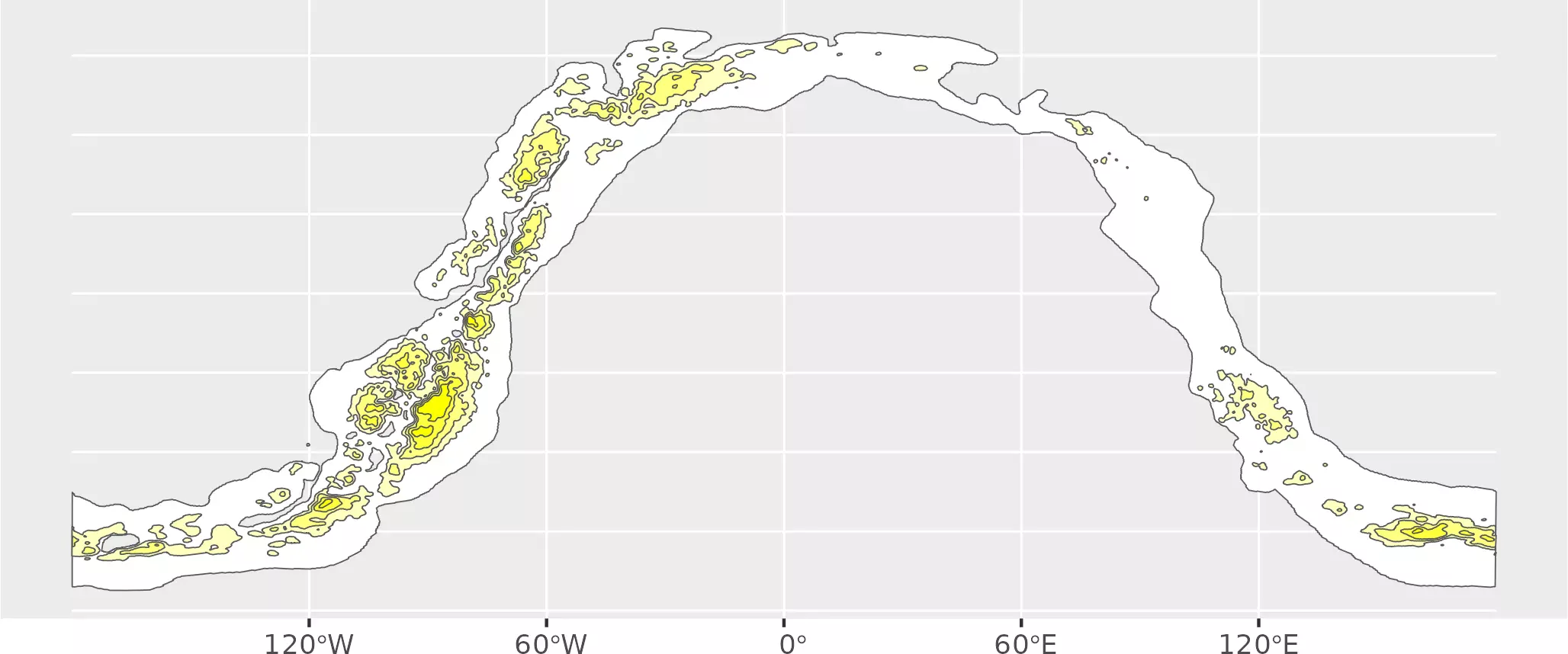
mw <- load_celestial("mw.min.geojson")

# Add colors to MW to use on fill
cols <- colorRampPalette(c("white", "yellow"))(5)
mw$fill <- factor(cols, levels = cols)

ggplot(mw) +
  geom_sf(aes(fill = fill)) +
  scale_fill_identity()

plot of chunk 20230125_mw

# And process it

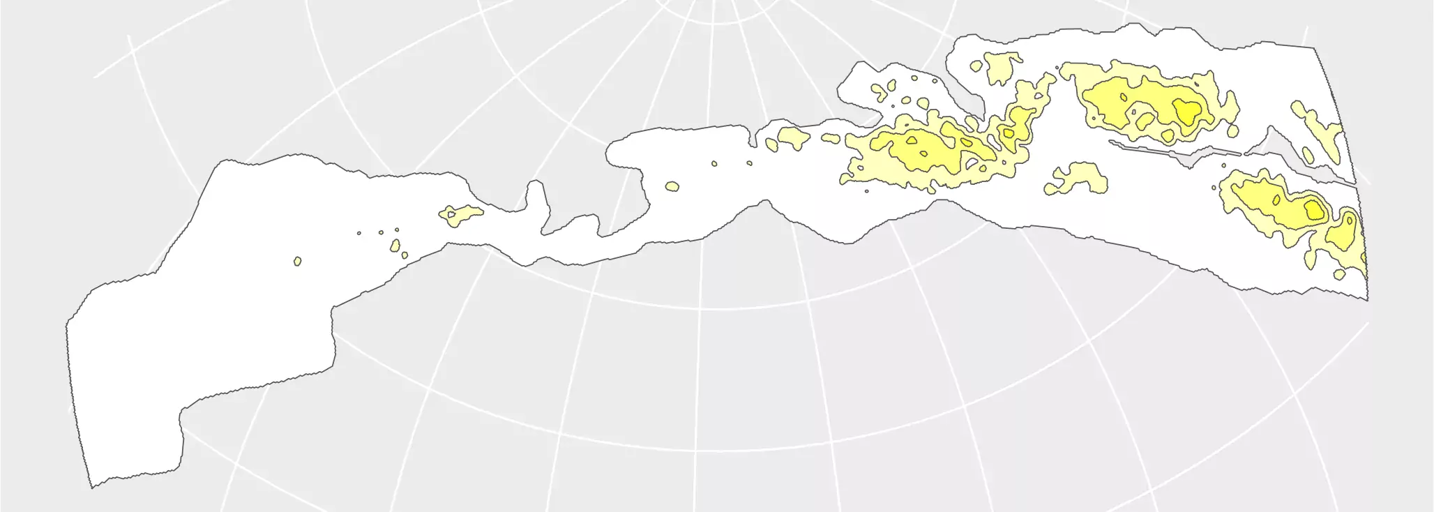
# Cut to buffer
mw_end <- sf_spherical_cut(mw,
  the_buff = hemisphere_s2,
  # Change the crs
  the_crs = target_crs,
  flip = flip_matrix
)


ggplot(mw_end) +
  geom_sf(aes(fill = fill)) +
  scale_fill_identity()

plot of chunk 20230125_mw

Now it is the turn of the constellations:

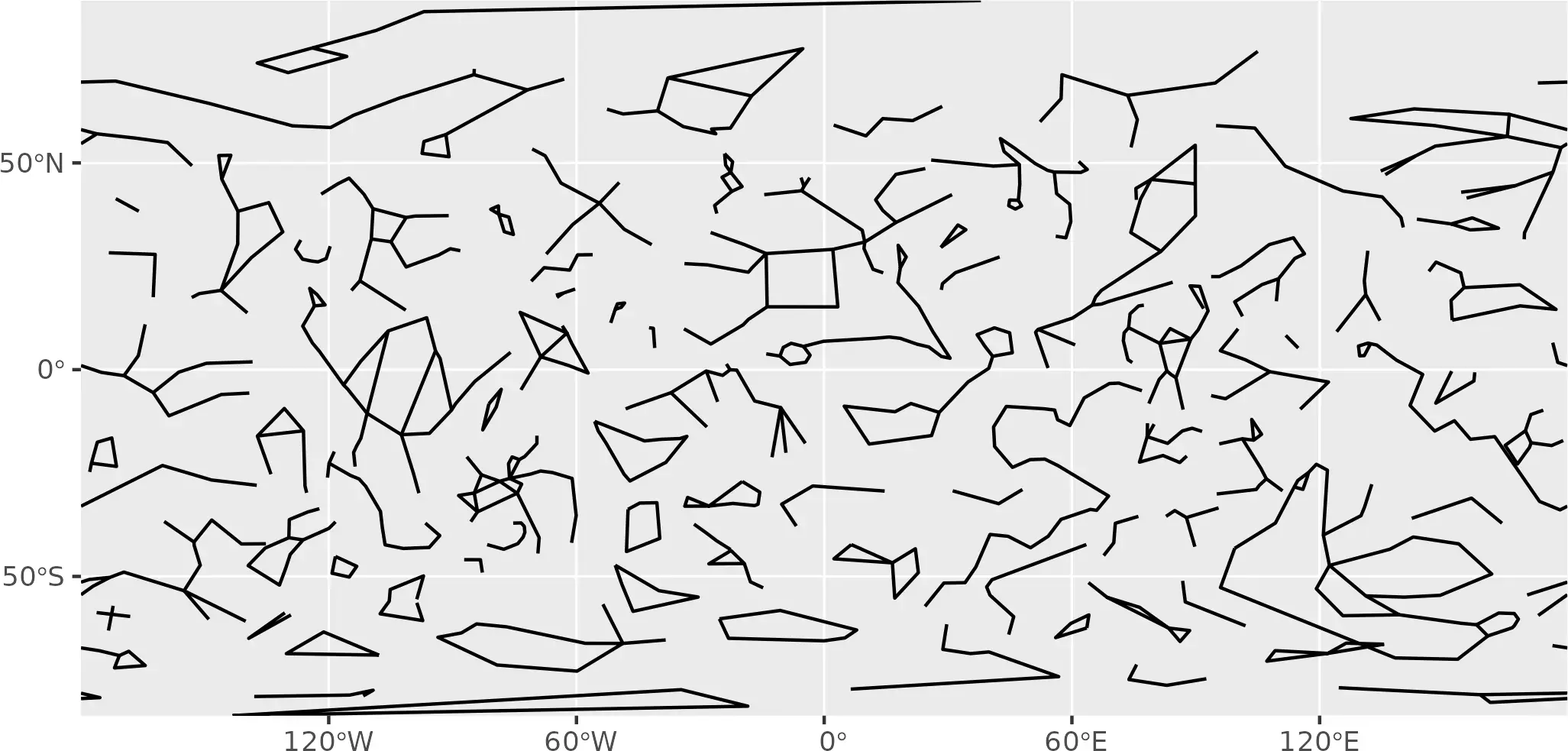
const <- load_celestial("constellations.lines.min.geojson")

ggplot(const) +
  geom_sf() +
  coord_sf(expand = FALSE)

plot of chunk 20230125_const

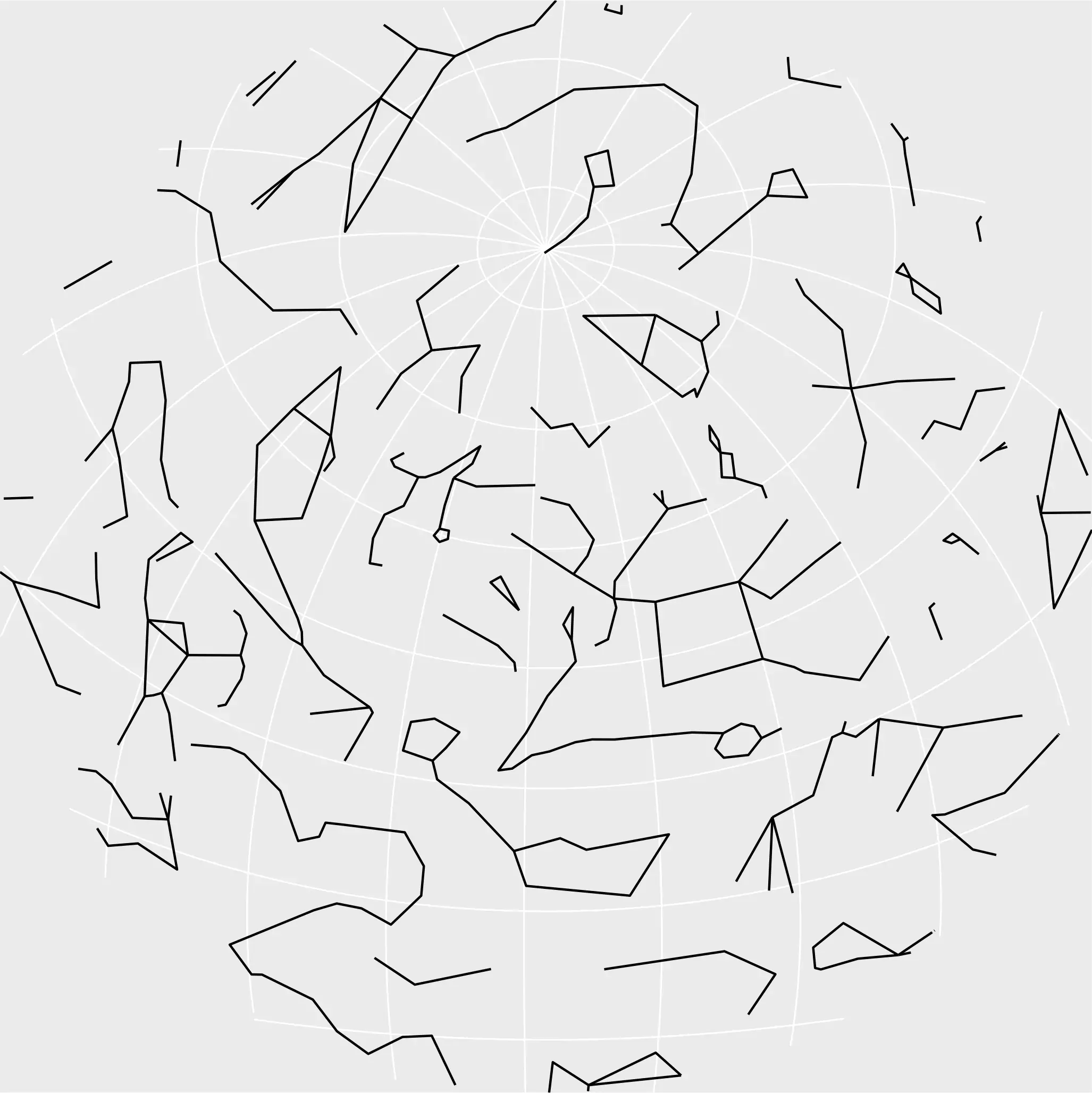
# Cut to buffer

const_end <- sf_spherical_cut(const,
  the_buff = hemisphere_s2,
  # Change the crs
  the_crs = target_crs,
  flip = flip_matrix
)


ggplot(const_end) +
  geom_sf() +
  coord_sf(expand = FALSE)

plot of chunk 20230125_const

And finally the stars:

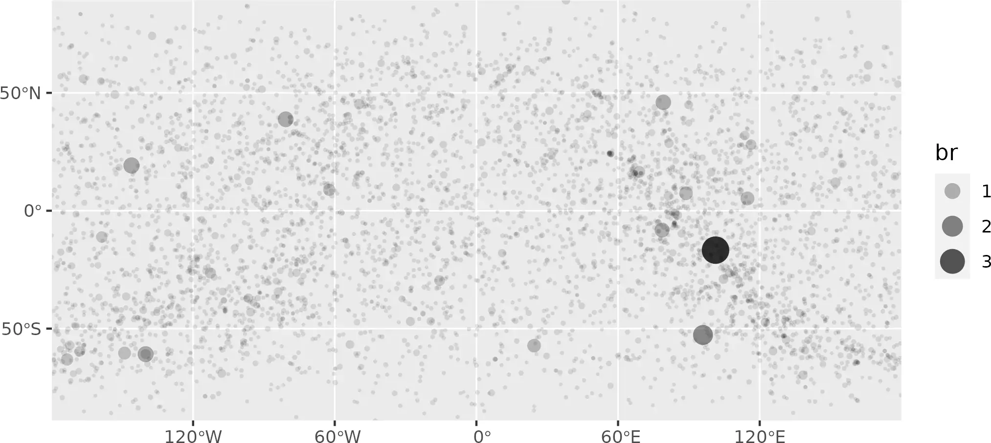
stars <- load_celestial("stars.6.min.geojson")

ggplot(stars) +
  # We use relative brightness (br) as aes
  geom_sf(aes(size = br, alpha = br), shape = 16) +
  scale_size_continuous(range = c(0.5, 6)) +
  scale_alpha_continuous(range = c(0.1, 0.8)) +
  coord_sf(expand = FALSE)

plot of chunk 20230125_stars

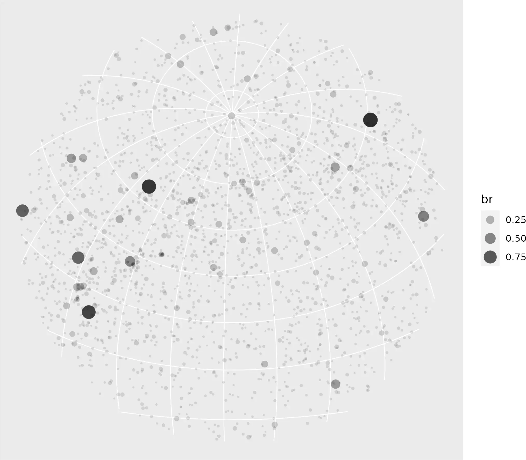
# Cut to buffer

stars_end <- sf_spherical_cut(stars,
  the_buff = hemisphere_s2,
  # Change the crs
  the_crs = target_crs,
  flip = flip_matrix
)

ggplot(stars_end) +
  # We use relative brightness (br) as aes
  geom_sf(aes(size = br, alpha = br), shape = 16) +
  scale_size_continuous(range = c(0.5, 6)) +
  scale_alpha_continuous(range = c(0.1, 0.8))

plot of chunk 20230125_stars

Graticules

We are going also to include graticules, so the Earth poles can be quickly spotted. In this case we don’t apply any affine transformation, so the flip parameter of sf_spherical_cut() needs to be set as NULL.

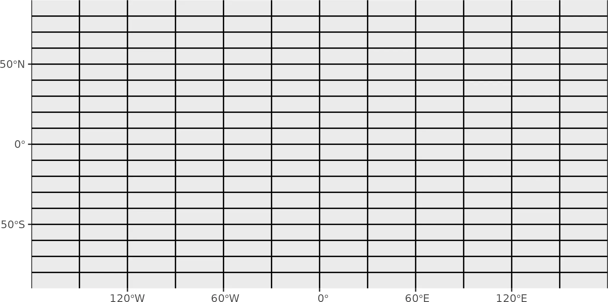
grat <- st_graticule(
  ndiscr = 5000,
  lat = seq(-90, 90, 10),
  lon = seq(-180, 180, 30)
)

ggplot(grat) +
  geom_sf() +
  coord_sf(expand = FALSE)

plot of chunk 20230125_grat

# Cut to buffer, we dont flip this one (it is not an object of the space)
grat_end <- sf_spherical_cut(
  x = grat,
  the_buff = hemisphere_s2,
  # Change the crs
  the_crs = target_crs
)


ggplot(grat_end) +
  geom_sf() +
  coord_sf(expand = FALSE)

plot of chunk 20230125_grat

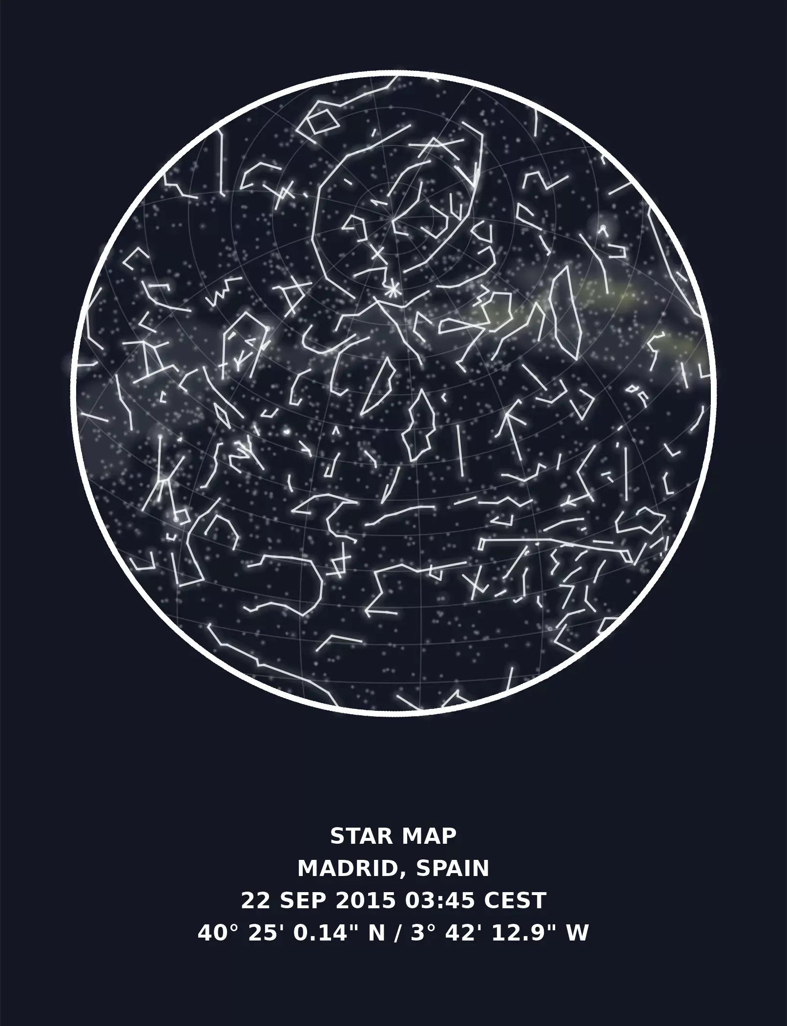
Visualization with `ggplot2`

We are almost set! For preparing the final map, first we are going to create the corresponding labels, that would be included as caption on the ggplot2 map:

lat_lab <- pretty_lonlat(desired_loc[1], type = "lat")
lon_lab <- pretty_lonlat(desired_loc[2], type = "lon")

pretty_labs <- paste(lat_lab, "/", lon_lab)

cat(pretty_labs)
#> 40° 25' 0.14" N / 3° 42' 12.9" W

# Create final caption to put on bottom

pretty_time <- paste(
  # Pretty Day
  scales::label_date(
    format = "%d %b %Y",
    locale = "en"
  )(desired_date_tz),
  # Pretty Hour
  format(desired_date_tz, format = "%H:%M", usetz = TRUE)
)

cat(pretty_time)
#> 22 Sep 2015 03:45 CEST

# Our final caption
caption <- toupper(paste0(
  "Star Map\n",
  desired_place, "\n",
  pretty_time, "\n",
  pretty_labs
))


cat(caption)
#> STAR MAP
#> MADRID, SPAIN
#> 22 SEP 2015 03:45 CEST
#> 40° 25' 0.14" N / 3° 42' 12.9" W

We can enhance the visualization by applying some interesting effects:

We want the Milky Way to appear a bit blurry instead of as a Well-Known geometry. With this effect we can mimic how we really see it from the Earth. So we can use ggfx::with_blur() to get this effect.
We can also add a glowing effect to our stars and constellations (have a look to Dominic Royé’s post Firefly Cartography to know more about this). The only drawback is that I was not able to use ggshadow with LINESTRING (Dominic shows how to do it with POINT), so instead I converted my lines (the constellations) to coordinates and applied ggshadow::geom_glowpath()

So we are ready now to create the final visualization:

# Prepare MULTILINESTRING

const_end_lines <- const_end %>%
  st_cast("MULTILINESTRING") %>%
  st_coordinates() %>%
  as.data.frame()


ggplot() +
  # Graticules
  geom_sf(data = grat_end, color = "grey60", linewidth = 0.25, alpha = 0.3) +
  # A blurry Milky Way
  with_blur(
    geom_sf(
      data = mw_end, aes(fill = fill), alpha = 0.1, color = NA,
      show.legend = FALSE
    ),
    sigma = 8
  ) +
  scale_fill_identity() +
  # Glowing stars
  geom_glowpoint(
    data = stars_end, aes(
      alpha = br, size =
        br, geometry = geometry
    ),
    color = "white", show.legend = FALSE, stat = "sf_coordinates"
  ) +
  scale_size_continuous(range = c(0.05, 0.75)) +
  scale_alpha_continuous(range = c(0.1, 0.5)) +
  # Glowing constellations
  geom_glowpath(
    data = const_end_lines, aes(X, Y, group = interaction(L1, L2)),
    color = "white", size = 0.5, alpha = 0.8, shadowsize = 0.4, shadowalpha = 0.01,
    shadowcolor = "white", linejoin = "round", lineend = "round"
  ) +
  # Border of the sphere
  geom_sf(data = hemisphere_sf, fill = NA, color = "white", linewidth = 1.25) +
  # Caption
  labs(caption = caption) +
  # And end with theming
  theme_void() +
  theme(
    text = element_text(colour = "white"),
    panel.border = element_blank(),
    plot.background = element_rect(fill = "#191d29", color = "#191d29"),
    plot.margin = margin(20, 20, 20, 20),
    plot.caption = element_text(
      hjust = 0.5, face = "bold",
      size = rel(1),
      lineheight = rel(1.2),
      margin = margin(t = 40, b = 20)
    )
  )

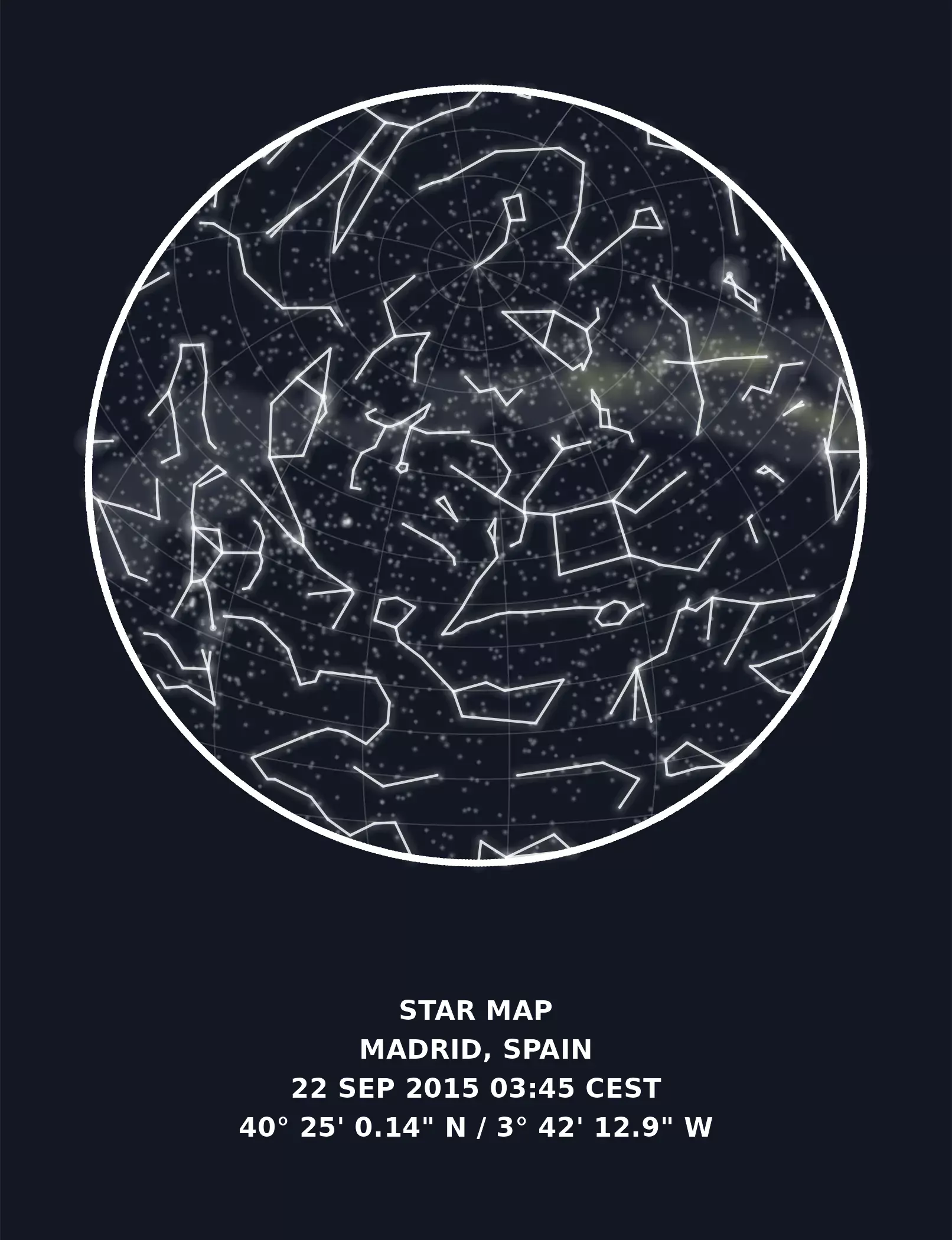
plot of chunk 20230125_celestial_map

Voilà! I checked several times the results with the results provided by d3-celestial.js on the location demo and the underlying calculations on Javascript and everything seems to be up and running.

Extra: Chinese constellations

Celestial Data also provides data for traditional Chinese constellations, so we can create a similar map with this whole different set of geometries:

const_cn <- load_celestial("constellations.lines.cn.min.geojson")

# Cut and prepare for geom_glowpath() on a single step
const_cn_end_lines <- sf_spherical_cut(const_cn,
  the_buff = hemisphere_s2,
  # Change the crs
  the_crs = target_crs,
  flip = flip_matrix
) %>%
  # To paths
  st_cast("MULTILINESTRING") %>%
  st_coordinates() %>%
  as.data.frame()


ggplot() +
  # Graticules
  geom_sf(data = grat_end, color = "grey60", linewidth = 0.25, alpha = 0.3) +
  # A blurry Milky Way
  with_blur(
    geom_sf(
      data = mw_end, aes(fill = fill), alpha = 0.1, color = NA,
      show.legend = FALSE
    ),
    sigma = 8
  ) +
  scale_fill_identity() +
  # Glowing stars
  geom_glowpoint(
    data = stars_end, aes(
      alpha = br, size =
        br, geometry = geometry
    ),
    color = "white", show.legend = FALSE, stat = "sf_coordinates"
  ) +
  scale_size_continuous(range = c(0.05, 0.75)) +
  scale_alpha_continuous(range = c(0.1, 0.5)) +
  # Glowing constellations
  geom_glowpath(
    data = const_cn_end_lines, aes(X, Y, group = interaction(L1, L2)),
    color = "white", size = 0.5, alpha = 0.8, shadowsize = 0.4, shadowalpha = 0.01,
    shadowcolor = "white", linejoin = "round", lineend = "round"
  ) +
  # Border of the sphere
  geom_sf(data = hemisphere_sf, fill = NA, color = "white", linewidth = 1.25) +
  # Caption
  labs(caption = caption) +
  # And end with theming
  theme_void() +
  theme(
    text = element_text(colour = "white"),
    panel.border = element_blank(),
    plot.background = element_rect(fill = "#191d29", color = "#191d29"),
    plot.margin = margin(20, 20, 20, 20),
    plot.caption = element_text(
      hjust = 0.5, face = "bold",
      size = rel(1),
      lineheight = rel(1.2),
      margin = margin(t = 40, b = 20)
    )
  )

plot of chunk 20230125_celestial_map_cn

References

Meeus J (1998). Astronomical algorithms, 2nd edition. Willmann-Bell, Richmond, Va. ISBN 9780943396613.

Frohn O, Hernangómez D (2023). “Celestial Data.” doi:10.5281/zenodo.7561601, https://dieghernan.github.io/celestial_data/.

Frohn O (2015). “d3-celestial.” https://github.com/ofrohn/d3-celestial/.

Fitter K (2019). “Celestial Maps.” (link).

Still J (2020). “Astronomical Calculations: Sidereal Time.” https://squarewidget.com/astronomical-calculations-sidereal-time/.

Pebesma E, Dunnington D (2020). “In r-spatial, the Earth is no longer flat.” (link).

Royé D (2020). “Firefly Cartography.” (link).

In fact, the download is performed via the jsDelivr, that distribute files hosted on GitHub via CDN. This is supposed to improve performance but in any case the underlying data source is the GitHub repo. ↑