Sometimes you want to produce maps with special layouts. I especially like maps with modified geometries, e.g. simplifying the original shapes to squares or dots. When searching the web, I found the fantastic post Fishnets and Honeycomb: Square vs. Hexagonal Spatial Grids by Matt Strimas-Mackey, which was a huge inspiration (by the way, don’t miss his blog, full of very interesting pieces of work).
The only thing I was not completely comfortable with was that the post used the old-fashioned sp package instead of my personal favorite, the sf package. The post was published in 2016, and note that the author has also moved to the sf package since then. So I decided to explore further options with sf.
The approach is similar, using grids over a map and working with them, but with
st_make_grid.
I also expanded it by grouping the grids and producing dots over the geometries.
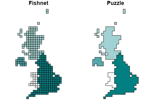
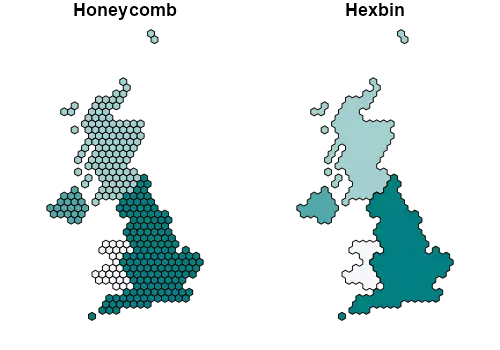
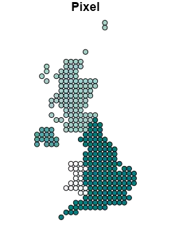
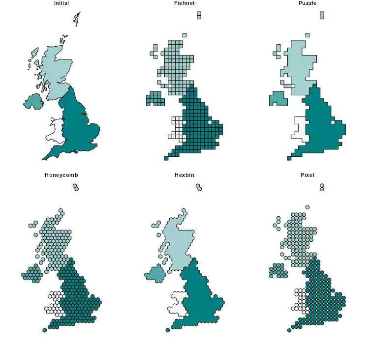
So basically I produced five variations of the map:
| Type | Replacement | Grouped |
|---|---|---|
| Fishnet | Square | No |
| Puzzle | Square | Yes |
| Honeycomb | Hexagon | No |
| Hexbin | Hexagon | Yes |
| Pixel | Dot | No |
Required R packages
library(sf)
library(giscoR)
library(dplyr)
library(RColorBrewer)
Working with square grids
Let’s use the square option of st_make_grid and play a bit with it.
GB <- ne_download(50,
  type = "map_subunits",
  returnclass = "sf",
  destdir = tempdir()
) %>%
  subset(CONTINENT == "Europe") %>%
  subset(ADM0_A3 == "GBR")

# Projecting and cleaning
GB <- st_transform(GB, 3857) %>% select(NAME_EN, ADM0_A3)
initial <- GB
initial$index_target <- 1:nrow(initial)
target <- st_geometry(initial)

# Create my own color palette
mypal <- colorRampPalette(c("#F3F8F8", "#008080"))
Warning: The cellsize should
be set in the same unit as the projection (in this case, meters). Pay special
attention to this because if the parameter is too small, meaning that the grid
is too dense, R could crash easily.
grid <- st_make_grid(target,
  50 * 1000,
  # Kms
  crs = st_crs(initial),
  what = "polygons",
  square = TRUE
)

# To sf
grid <- st_sf(index = 1:length(lengths(grid)), grid) # Add index

# We identify the grids that belong to an entity by assessing the centroid
cent_grid <- st_centroid(grid)
cent_merge <- st_join(cent_grid, initial["index_target"], left = F)
grid_new <- inner_join(grid, st_drop_geometry(cent_merge))

# Fishnet
Fishgeom <- aggregate(grid_new,
  by = list(grid_new$index_target),
  FUN = min,
  do_union = FALSE
)

# Let's add the data frame
Fishnet <- left_join(
  Fishgeom %>% select(index_target),
  st_drop_geometry(initial)
) %>%
  select(-index_target)

# Now let's create the puzzle
Puzzlegeom <- aggregate(st_buffer(grid_new, 0.5), # Avoid slivers
  by = list(grid_new$index_target),
  FUN = min,
  do_union = TRUE
) # This changes!!!

Puzzle <- left_join(
  Puzzlegeom %>% select(index_target),
  st_drop_geometry(initial)
) %>%
  select(-index_target)

# Plot
par(mfrow = c(1, 2), mar = c(1, 1, 1, 1), bg = NA)
plot(st_geometry(Fishnet), col = mypal(4), main = "Fishnet")
plot(st_geometry(Puzzle), col = mypal(4), main = "Puzzle")
Going hex
Extremely easy. We just need to change the square parameter of
st_make_grid from TRUE to FALSE.
grid <- st_make_grid(target,
  50 * 1000, # Kms
  crs = st_crs(initial),
  what = "polygons",
  square = FALSE # This is the only piece that changes!!!
)
# Make sf
grid <- st_sf(index = 1:length(lengths(grid)), grid) # Add index

# We identify the grids that belong to an entity by assessing the centroid
cent_grid <- st_centroid(grid)
cent_merge <- st_join(cent_grid, initial["index_target"], left = F)
grid_new <- inner_join(grid, st_drop_geometry(cent_merge))

# Honeycomb
Honeygeom <- aggregate(
  grid_new,
  by = list(grid_new$index_target),
  FUN = min,
  do_union = FALSE
)

# Let's add the data frame
Honeycomb <- left_join(
  Honeygeom %>%
    select(index_target),
  st_drop_geometry(initial)
) %>%
  select(-index_target)

# Now let's create the hexbin

Hexbingeom <- aggregate(
  st_buffer(grid_new, 0.5), # Avoid slivers
  by = list(grid_new$index_target),
  FUN = min,
  do_union = TRUE
)

Hexbin <- left_join(
  Hexbingeom %>%
    select(index_target),
  st_drop_geometry(initial)
) %>%
  select(-index_target)

# Plot
par(mfrow = c(1, 2), mar = c(1, 1, 1, 1), bg = NA)
plot(st_geometry(Honeycomb), col = mypal(4), main = "Honeycomb")
plot(st_geometry(Hexbin), col = mypal(4), main = "Hexbin")
Pixel it!
Also quite easy, just a couple more tweaks, still using st_make_grid.
grid <- st_make_grid(target,
  50 * 1000, # Kms
  crs = st_crs(initial),
  what = "centers"
)

# Make sf
grid <- st_sf(index = 1:length(lengths(grid)), grid) # Add index

# We identify the grids that belong to an entity by assessing the centroid
cent_grid <- st_centroid(grid)
cent_merge <- st_join(cent_grid, initial["index_target"], left = F)
grid_new <- st_buffer(cent_merge, 50 * 1000 / 2)
Pixelgeom <- aggregate(
  grid_new,
  by = list(grid_new$index_target),
  FUN = min,
  do_union = FALSE
)
# Let's add the data frame
Pixel <- left_join(
  Pixelgeom %>%
    select(index_target),
  st_drop_geometry(initial)
) %>%
  select(-index_target)

# Plot
par(mfrow = c(1, 1), mar = c(1, 1, 1, 1), bg = NA)
plot(st_geometry(Pixel), col = mypal(4), main = "Pixel")
Wrap up
Finally, I wrapped all that in a function named stdh_gridpol. See the code in
my repo:
stdh_gridpol <- function(sf,
                         to = "fishnet",
                         gridsize = as.integer(
                           min(
                             diff(st_bbox(sf)[c(1, 3)]),
                             diff(st_bbox(sf)[c(2, 4)])
                           ) / 40
                         ),
                         sliver = 0.5) {
  if (!unique(st_geometry_type(sf)) %in% c("POLYGON", "MULTIPOLYGON")) {
    stop("Input should be MULTIPOLYGON or POLYGON")
  }
  if (!to %in% c("fishnet", "puzzle", "honeycomb", "hexbin", "pixel")) {
    stop("'to' should be 'fishnet','puzzle','honeycomb','hexbin' or 'pixel'")
  }

  if (class(sf)[1] == "sf") {
    initial <- sf
    initial$index_target <- 1:nrow(initial)
  } else {
    initial <- st_sf(index_target = 1:length(sf), geom = sf)
  }

  target <- st_geometry(initial)

  if (to %in% c("fishnet", "puzzle")) {
    sq <- T
  } else {
    sq <- F
  }
  if (to == "pixel") {
    grid <- st_make_grid(target,
      gridsize,
      crs = st_crs(initial),
      what = "centers"
    )
  } else {
    grid <- st_make_grid(
      target,
      gridsize,
      crs = st_crs(initial),
      what = "polygons",
      square = sq
    )
  }
  grid <- st_sf(index = 1:length(lengths(grid)), grid) # Add index
  if (to == "pixel") {
    cent_merge <- st_join(grid, initial["index_target"], left = F)
    grid_new <- st_buffer(cent_merge, gridsize / 2)
  } else {
    cent_grid <- st_centroid(grid)
    cent_merge <- st_join(cent_grid, initial["index_target"], left = F)
    grid_new <- inner_join(grid, st_drop_geometry(cent_merge))
  }
  if (to %in% c("fishnet", "honeycomb", "pixel")) {
    geom <- aggregate(
      grid_new,
      by = list(grid_new$index_target),
      FUN = min,
      do_union = FALSE
    )
  } else {
    geom <- aggregate(
      st_buffer(grid_new, sliver),
      by = list(grid_new$index_target),
      FUN = min,
      do_union = TRUE
    )
  }
  if (class(initial)[1] == "sf") {
    fin <- left_join(
      geom %>% select(index_target),
      st_drop_geometry(initial)
    ) %>%
      select(-index_target)
    fin <- st_cast(fin, "MULTIPOLYGON")
    return(fin)
  } else {
    fin <- st_cast(geom, "MULTIPOLYGON")
    return(st_geometry(fin))
  }
}
# End of the function-----

fish <- stdh_gridpol(GB, to = "fishnet", gridsize = 50 * 1000)
puzz <- stdh_gridpol(GB, to = "puzzle", gridsize = 50 * 1000)
hon <- stdh_gridpol(GB, to = "honeycomb", gridsize = 50 * 1000)
hex <- stdh_gridpol(GB, to = "hexbin", gridsize = 50 * 1000)
pix <- stdh_gridpol(GB, to = "pixel", gridsize = 50 * 1000)
And that’s it! The function stdh_gridpol has some alert mechanisms, such as
accepting only POLYGON or MULTIPOLYGON, and the default value of gridsize
is computed so that the shortest dimension has 40 cells.