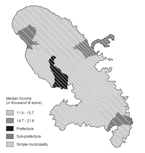
In this post, I show how to produce different filling patterns that can be added over your shapefiles with the cartography package.
Historical example: The mapping examples use cartography, which is now in maintenance mode. Its maintainers recommend mapsf for new work. The original code and outputs are preserved and have not been revalidated against current package versions.
Updated 17 February 2020: All these pieces of work are already available
in cartography >v.2.4.0 through the hatchedLayer
and legendHatched
functions. Just install it via install.packages("cartography"). A dedicated
blog post with examples is available at this link.
Required R packages
library(sf)
library(dplyr)
library(giscoR)
library(cartography)
DE <- gisco_get_countries(country = "Germany", epsg = 3857)
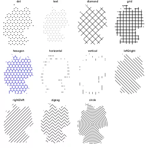
Let’s see how it works.
par(
  mfrow = c(3, 4),
  mar = c(1, 1, 1, 1),
  cex = 0.5
)
hatchedLayer(DE, "dot")
title("dot")
hatchedLayer(DE, "text", txt = "Y")
title("text")
hatchedLayer(DE, "diamond", density = 0.5)
title("diamond")
hatchedLayer(DE, "grid", lwd = 1.5)
title("grid")
hatchedLayer(DE, "hexagon", col = "blue")
title("hexagon")
hatchedLayer(DE, "horizontal", lty = 5)
title("horizontal")
hatchedLayer(DE, "vertical")
title("vertical")
hatchedLayer(DE, "left2right")
title("left2right")
hatchedLayer(DE, "right2left")
title("right2left")
hatchedLayer(DE, "zigzag")
title("zigzag")
hatchedLayer(DE, "circle")
title("circle")
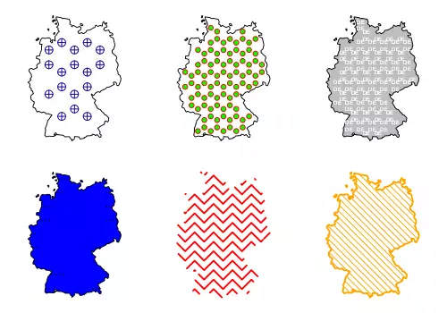
Let’s play a little bit more with some of the additional features of the function:
par(mar = c(1, 1, 1, 1), mfrow = c(2, 3))
plot(st_geometry(DE))
hatchedLayer(
  DE,
  "dot",
  pch = 10,
  density = 0.5,
  cex = 2,
  col = "darkblue",
  add = T
)
plot(st_geometry(DE))
hatchedLayer(
  DE,
  "dot",
  pch = 21,
  col = "red",
  bg = "green",
  cex = 1.25,
  add = T
)
plot(st_geometry(DE), col = "grey")
hatchedLayer(
  DE,
  "text",
  txt = "DE",
  density = 1.1,
  col = "white",
  add = T
)
plot(st_geometry(DE), col = "blue")
hatchedLayer(
  DE,
  "horizontal",
  lty = 3,
  cellsize = 150 * 1000,
  add = T
)
hatchedLayer(DE, "zigzag", lwd = 2, col = "red")
plot(st_geometry(DE), border = "orange", lwd = 2)
hatchedLayer(DE,
  "left2right",
  density = 2,
  col = "orange",
  add = T
)
Adding legends: the legendHatched function
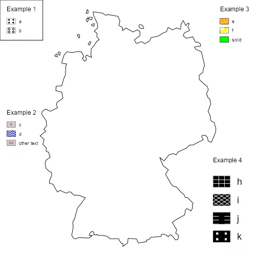
As a complementary function, there is also legendHatched. The main parameters
are:
pos,title.txt,title.cex,values.cex,categ,cexandframe: See?cartography::legendTypo.patterns: Vector of patterns to be created for each element oncateg.ptrn.bg: Background of the legend box for eachcateg.ptrn.text: Text to be used for eachcateg="text", as a single value or a vector.dot.cex:cexof eachcateg="dot", as a single value or a vector.text.cex: Text size of eachcateg="text", as a single value or a vector.- As in the case of the
hatchedLayerfunction, different graphical parameters can be passed (lty,lwd,pch,bgon points).
Note that it is also possible to create solid legends by setting col and
ptrn.bg to the same color. Parameters respect the order of the categ
variable.
par(mar = c(0, 0, 0, 0), mfrow = c(1, 1))
plot(st_geometry(DE)) # Null geometry
legendHatched(
  title.txt = "Example 1",
  categ = c("a", "b"),
  patterns = "dot",
  pch = c(16, 23),
  frame = T
)
legendHatched(
  pos = "left",
  title.txt = "Example 2",
  categ = c("c", "d", "other text"),
  patterns = c("text", "zigzag"),
  ptrn.text = c("s", "pp"),
  ptrn.bg = "grey80",
  col = c("red", "blue")
)

legendHatched(
  pos = "topright",
  title.txt = "Example 3",
  categ = c("e", "f", "solid"),
  patterns = c("circle", "left2right"),
  ptrn.bg = c("orange", "yellow", "green"),
  col = c("white", "white", "green"),
  lty = c(2, 4),
  lwd = c(1, 3)
)


legendHatched(
  pos = "bottomright",
  title.txt = "Example 4",
  values.cex = 1.2,
  categ = c("h", "i", "j", "k"),
  patterns = c("grid", "diamond", "horizontal", "dot"),
  cex = 2,
  pch = 22,
  col = "white",
  ptrn.bg = "black",
  bg = "pink"
)
I hope that you find these functions useful. Enjoy, and happy mapping!