How to place an inset map in R? There are many solutions out there using the ggplot2 package (see Drawing beautiful maps programmatically with R, sf and ggplot2 by Mel Moreno and Mathieu Basille). However, I like the old reliable plot function, so the question is: is there another way?
There is. I found inspiration here and I just applied it to a map.
Required R packages
library(sf)
library(dplyr)
library(rnaturalearth)
Mimicking Moreno & Basille
I would present here an alternative version of Drawing beautiful maps programmatically with R, sf and ggplot2, so the bulk of the detail can be found there. I would focus only in the plot()side.
world <- ne_countries(scale = "medium", returnclass = "sf")
USA <- subset(world, admin == "United States of America")
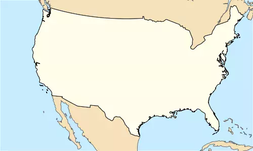
# Plot mainland USA----
par(mar = c(0, 0, 0, 0))
plot(
st_geometry(world %>%
st_transform(2163)),
xlim = c(-2500000, 2500000),
ylim = c(-2300000, 730000),
col = "#F6E1B9",
border = "#646464",
bg = "#C6ECFF"
)
plot(
st_geometry(USA) %>% st_transform(2163),
col = "#FEFEE9",
border = "black",
add = T
)
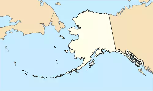
# Plot Alaska----
plot(
  st_geometry(world %>%
    st_transform(3467)),
  xlim = c(-2400000, 1600000),
  ylim = c(200000, 2500000),
  col = "#F6E1B9",
  border = "#646464",
  bg = "#C6ECFF"
)
plot(
  st_geometry(USA) %>% st_transform(3467),
  col = "#FEFEE9",
  border = "black",
  add = T
)
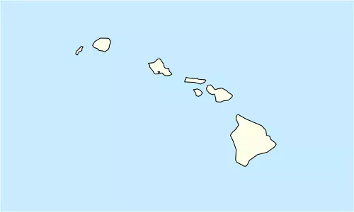
# Plot Hawaii----
plot(
  st_geometry(world %>%
    st_transform(4135)),
  xlim = c(-161, -154),
  ylim = c(18, 23),
  col = "#F6E1B9",
  border = "#646464",
  bg = "#C6ECFF"
)
plot(
  st_geometry(USA) %>% st_transform(4135),
  col = "#FEFEE9",
  border = "black",
  add = T
)
Insetting
From now on, I just focus on the inset part, using the fig() option on par(). Quoting statmethods:
(…) think of the full graph area as going from
(0,0)in the lower left corner to(1,1)in the upper right corner. The format of thefig=parameter is a numerical vector of the formc(x1, x2, y1, y2)(…)fig=starts a new plot, so to add to an existing plot usenew=TRUE.
So being x1 and y1 the starting points and x2, y2 the final points, we just can set up those parameters and adjust the final placement of the insets. Additionally I added a box around the insets using bbox(). I didn’t mimic Moreno & Basille here and I just worked it by myself.
par(mar = c(0, 0, 0, 0))
plot(
  st_geometry(world %>%
    st_transform(2163)),
  xlim = c(-2500000, 2500000),
  ylim = c(-2300000, 730000),
  col = "#F6E1B9",
  border = "#646464",
  bg = "#C6ECFF"
)
plot(
  st_geometry(USA) %>% st_transform(2163),
  col = "#FEFEE9",
  border = "black",
  add = T
)
# Alaska
par(
  fig = c(0.01, 0.28, 0.01, 0.33),
  new = TRUE
)
plot(
  st_geometry(world %>%
    st_transform(3467)),
  xlim = c(-2400000, 1600000),
  ylim = c(200000, 2500000),
  col = "#F6E1B9",
  border = "#646464",
  bg = "#C6ECFF"
)
plot(
  st_geometry(USA) %>% st_transform(3467),
  col = "#FEFEE9",
  border = "black",
  add = T
)
box(which = "figure", lwd = 1)

# Hawaii
par(
  fig = c(0.29, 0.45, 0.01, 0.15),
  new = TRUE
)
plot(
  st_geometry(world %>%
    st_transform(4135)),
  xlim = c(-161, -154),
  ylim = c(18, 23),
  col = "#F6E1B9",
  border = "#646464",
  bg = "#C6ECFF"
)
plot(
  st_geometry(USA) %>% st_transform(4135),
  col = "#FEFEE9",
  border = "black",
  add = T
)

box(which = "figure", lwd = 1)
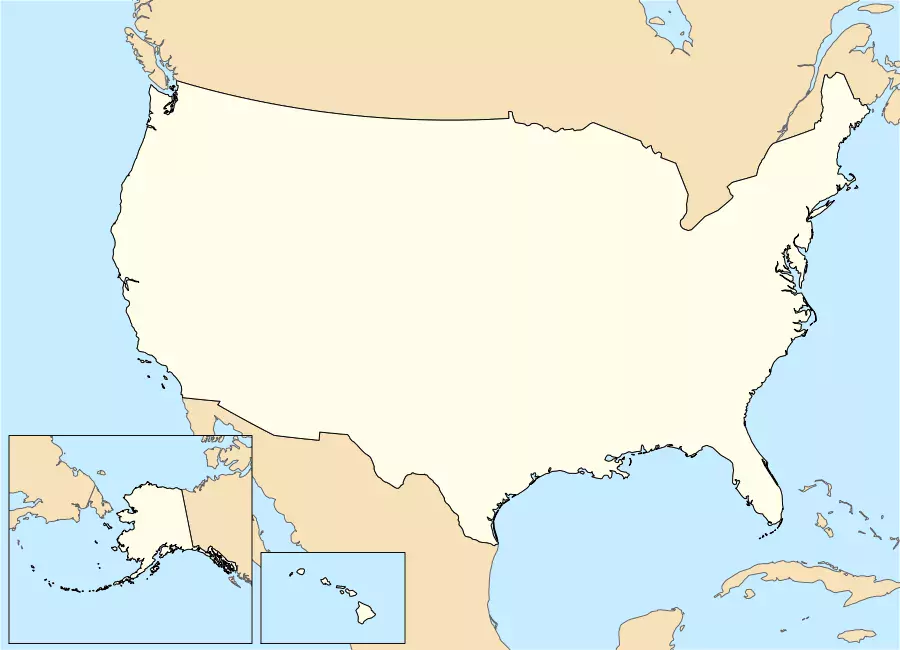
Results may vary depending of the size of the original plot (Mainland USA) and your plotting device and output. However with a bit of trial-and-error it is quite easy to adjust the final result.
As an example, see one of my contributions to Wikimedia Commons that represents a map of the NUTS3 regions of the European Union. Several countries (France, Portugal, Spain) have overseas territories so I made a few insets on the right side.
