Getting started with rasterpic is straightforward: you need an image file (png, jpeg/jpg or tiff/tif) and a supported spatial input class, such as an object from the sf, terra or stars packages.
Basic usage
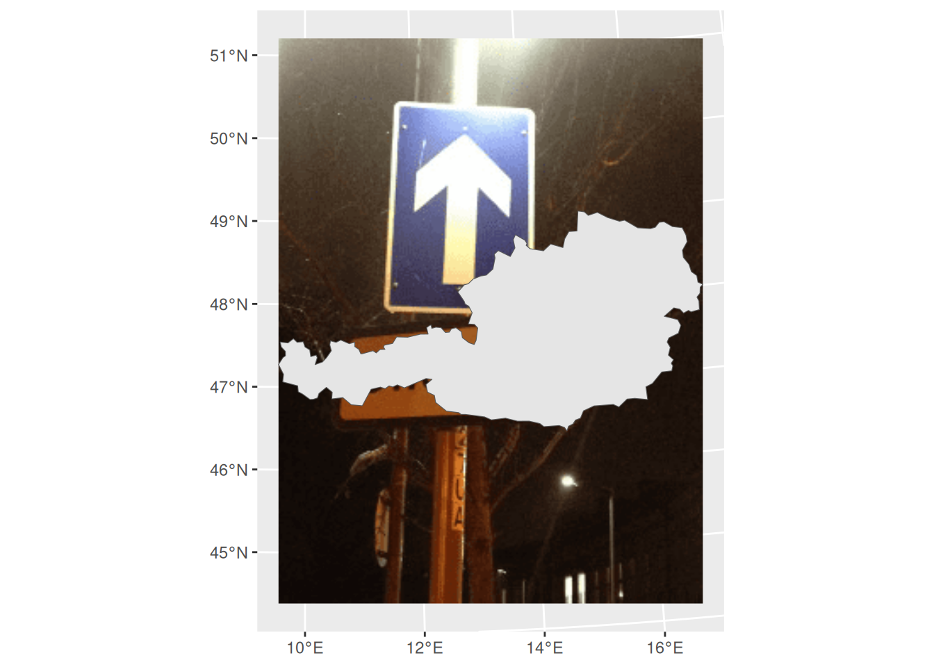
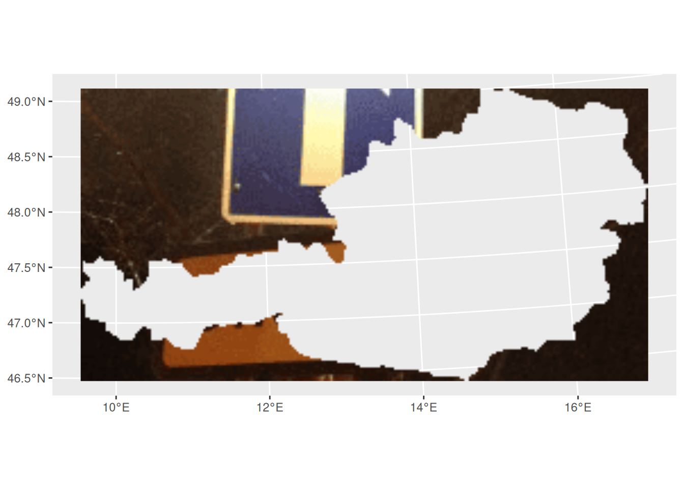
This example geotags an image using the shape of Austria:
Options
rasterpic_img() provides options for expansion, alignment, cropping and masking.
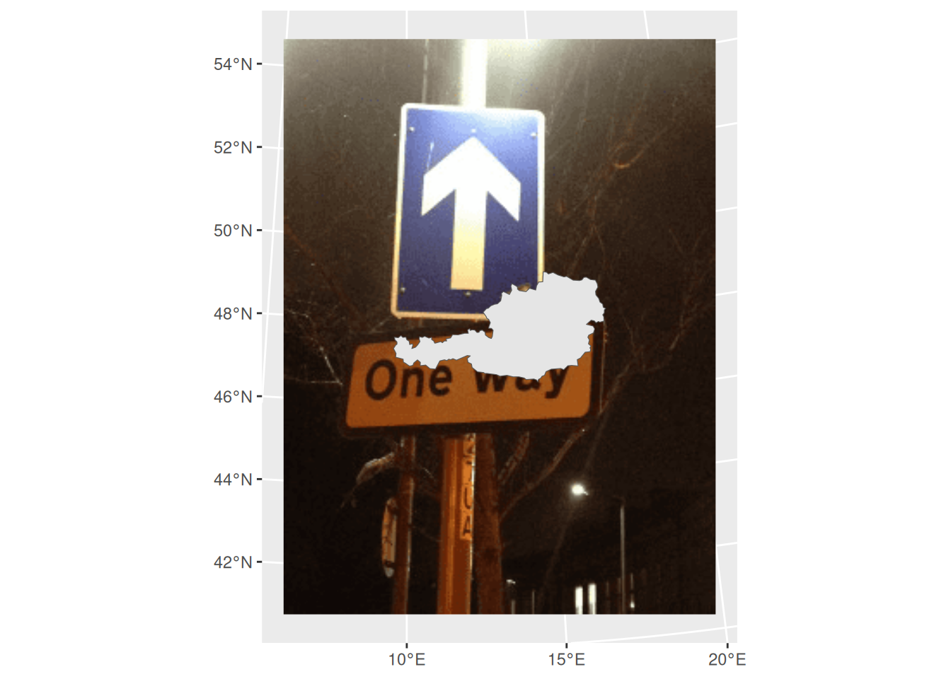
Expand
The expand argument expands the raster extent beyond the spatial object:
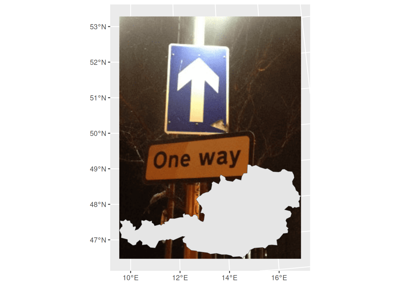
Alignment
The halign and valign arguments control the alignment of the image within the spatial extent:
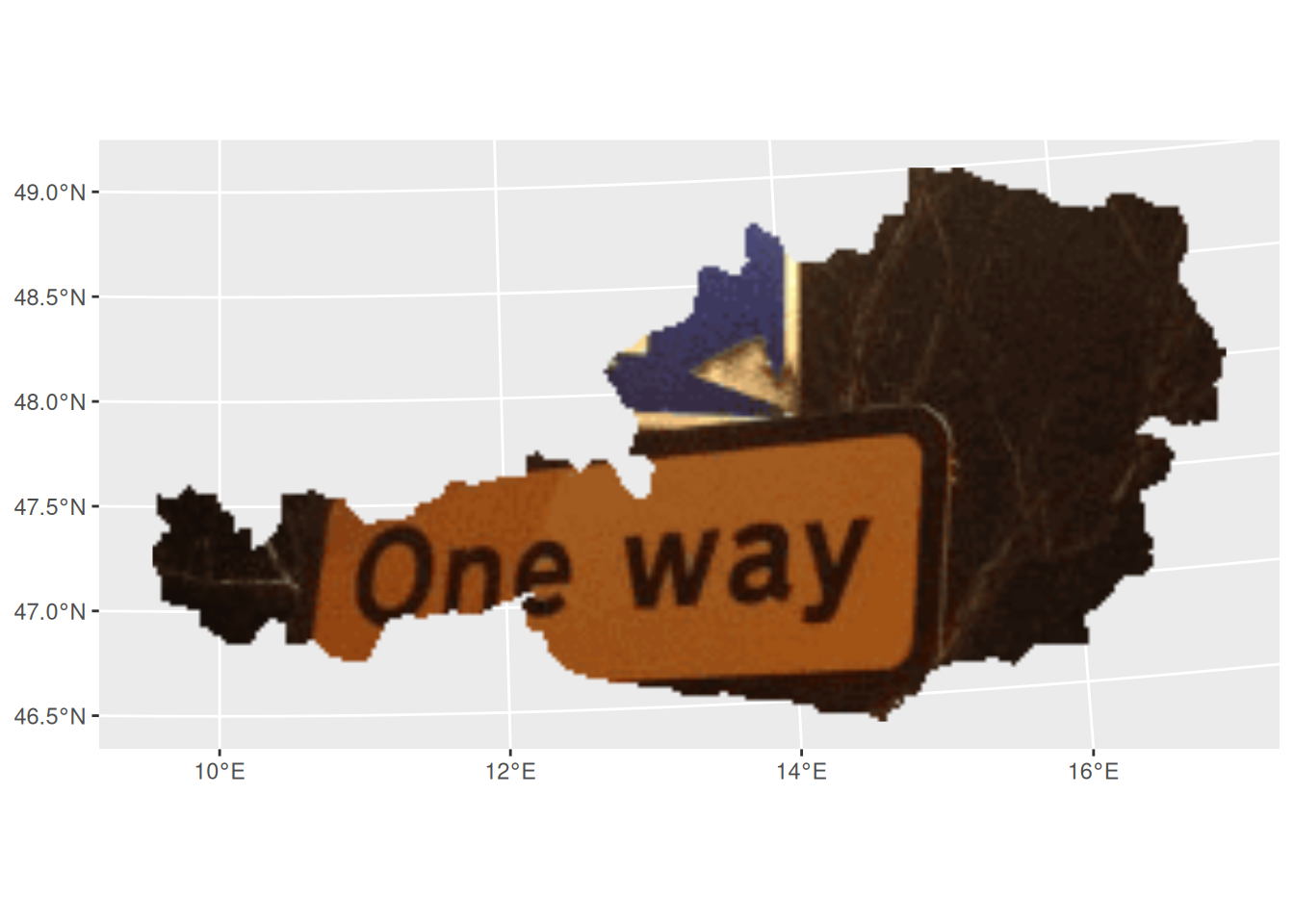
Crop and mask
The crop, mask and inverse arguments control whether the raster is cropped to the object extent and masked to the object shape:
rasterpic_img() supports the following spatial input classes:
-
sf classes:
sf, sfc, sfg and bbox.
-
terra classes:
SpatRaster, SpatVector and SpatExtent.
-
stars class:
stars.
- A numeric coordinate vector of the form
c(xmin, ymin, xmax, ymax).
rasterpic_img() is an S3 generic. Methods for extent-like inputs use the object extent, and vector methods can also mask the image to the object shape.
rasterpic can read the following image formats:
-
png files.
-
jpeg/jpg files.
-
tiff/tif files.