If you have been playing around with R for a while, you are probably
familiar with the volcano dataset:
data("volcano")
image(volcano, col = terrain.colors(256, rev = TRUE))
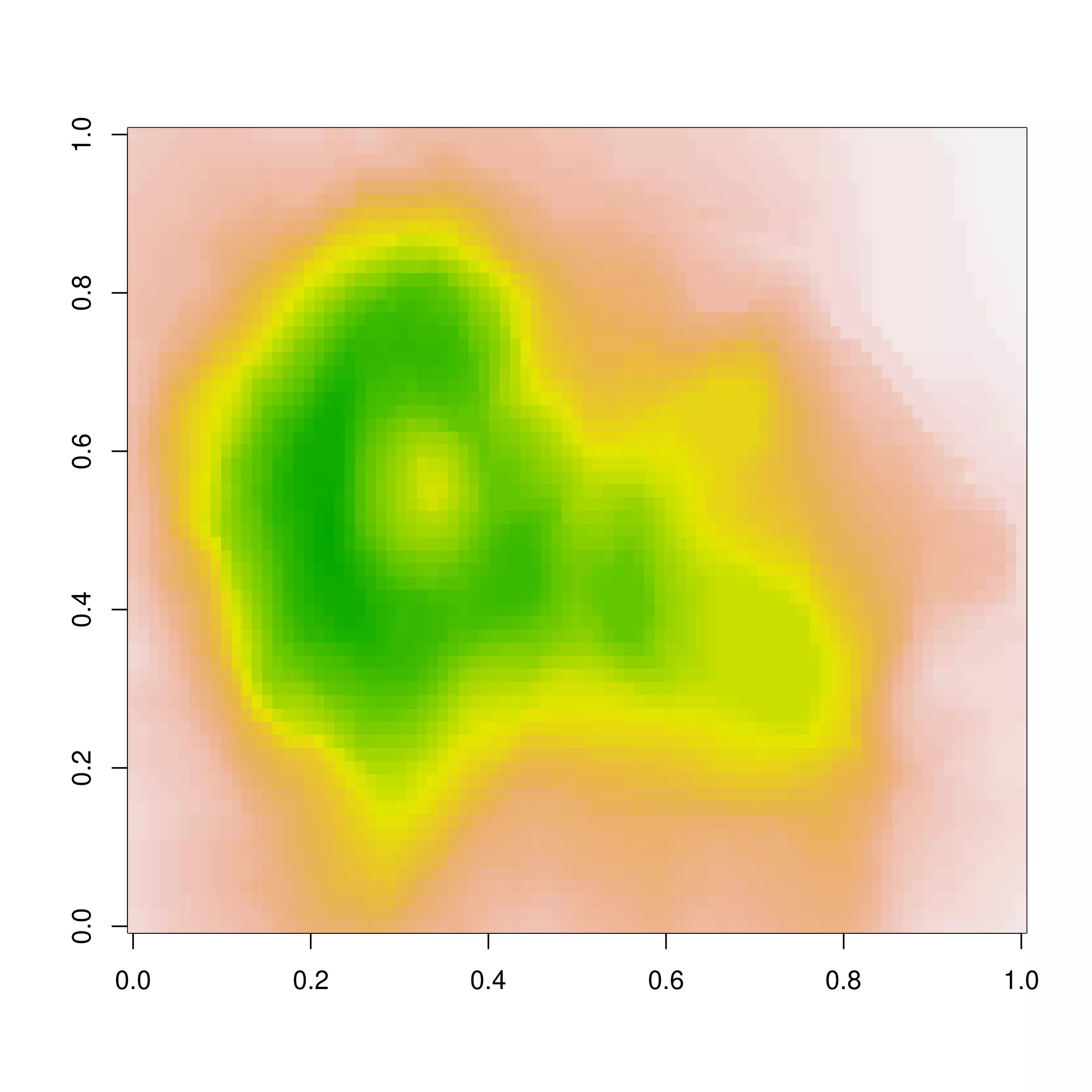
This represents the topographic information about one of the volcanoes of Auckland (New Zealand), specifically Maungawhau / Mount Eden. But do you know that this map is flipped?
In this post I introduce the tidyterra
package, recently added to
CRAN, and I show you how to
geotag the volcano dataset. We will also produce ggplot2 maps using the
functions of tidyterra.
# Libraries
library(terra)
library(ggplot2)
library(tidyterra)
library(maptiles)
library(sf)
Wait, volcano is flipped?
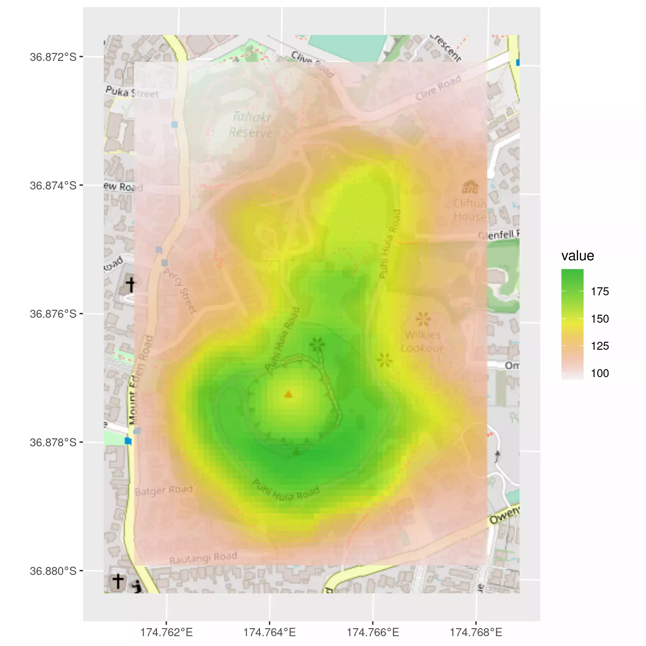
Let’s check it out. Thanks to the package maptiles we can have a glimpse of the location of Maungawhau using map tiles, as in Google Maps. We will use tidyterra for displaying the map tile:
# location of Maungawhau

box <- c(
  174.7611552780,
  -36.8799200525,
  174.7682380109,
  -36.8719519780
)
class(box) <- "bbox"
box <- st_as_sfc(box)
st_crs(box) <- 4326

box <- box %>%
  # To crs for NZGD49
  st_transform(27200)

tile <- get_tiles(box, crop = TRUE, zoom = 16)


ggtile <- ggplot() +
  geom_spatraster_rgb(data = tile)

ggtile
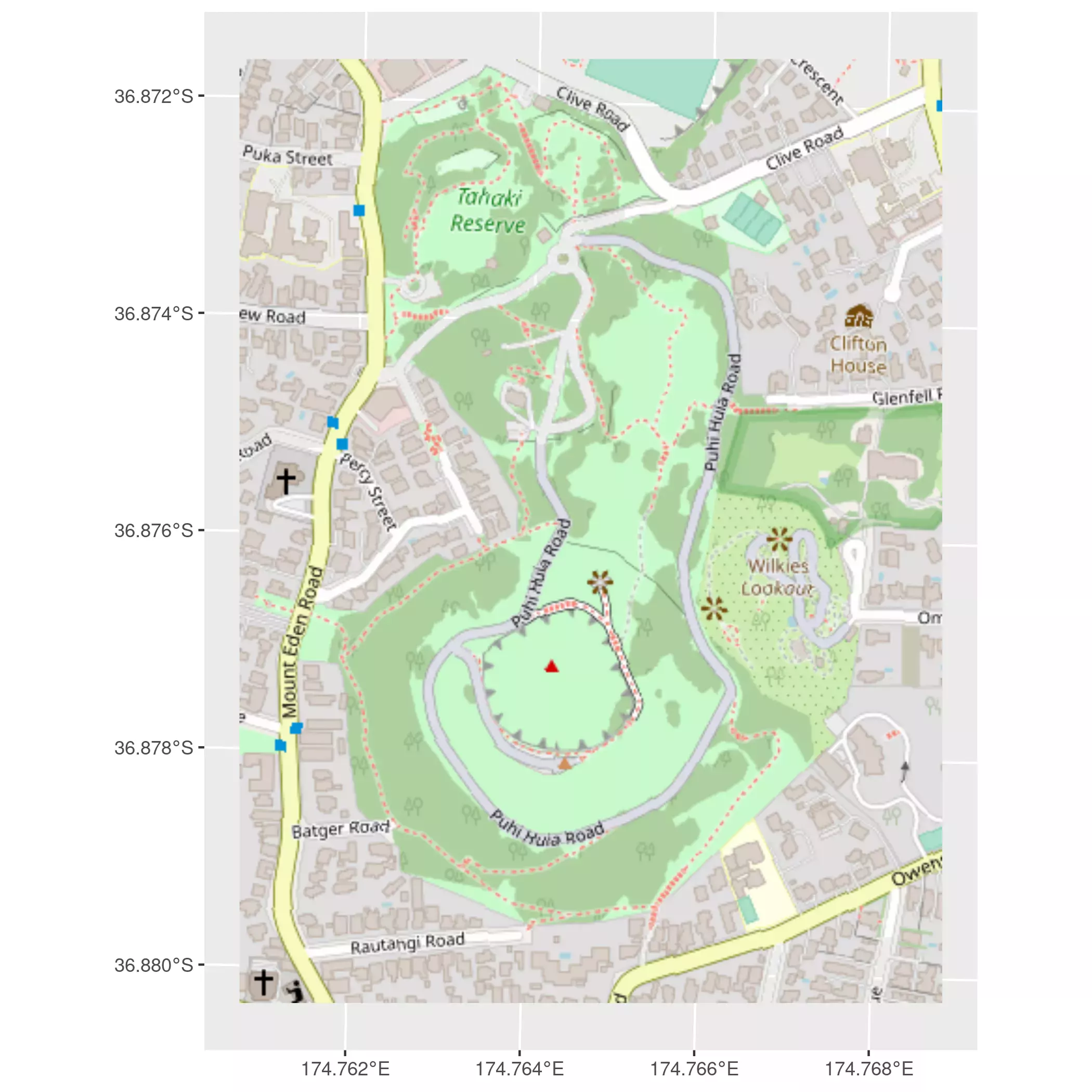
Here we have a crisp RGB tile of Maungawhau. Now, the next
question is how to match the volcano dataset (a matrix) with this tile (a
geotagged map tile)? Let’s check it out.
Working with SpatRasters
Thanks to the terra package we can start converting volcano into a
SpatRaster:
volcano_rast <- rast(volcano)

terra::plot(volcano_rast)
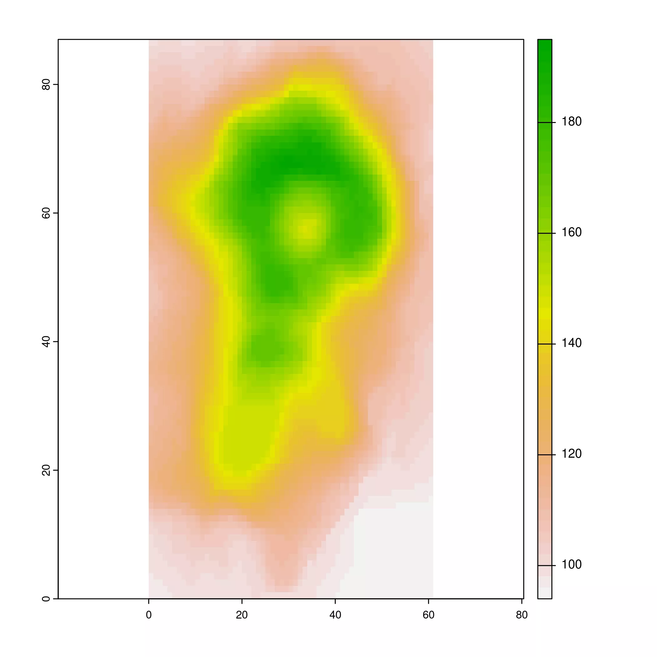
# Wait, it is flipped!
volcano_rast_ok <- rast(volcano[
  seq(nrow(volcano), 1, -1),
  seq(ncol(volcano), 1, -1)
])

# Much better!
terra::plot(volcano_rast_ok)
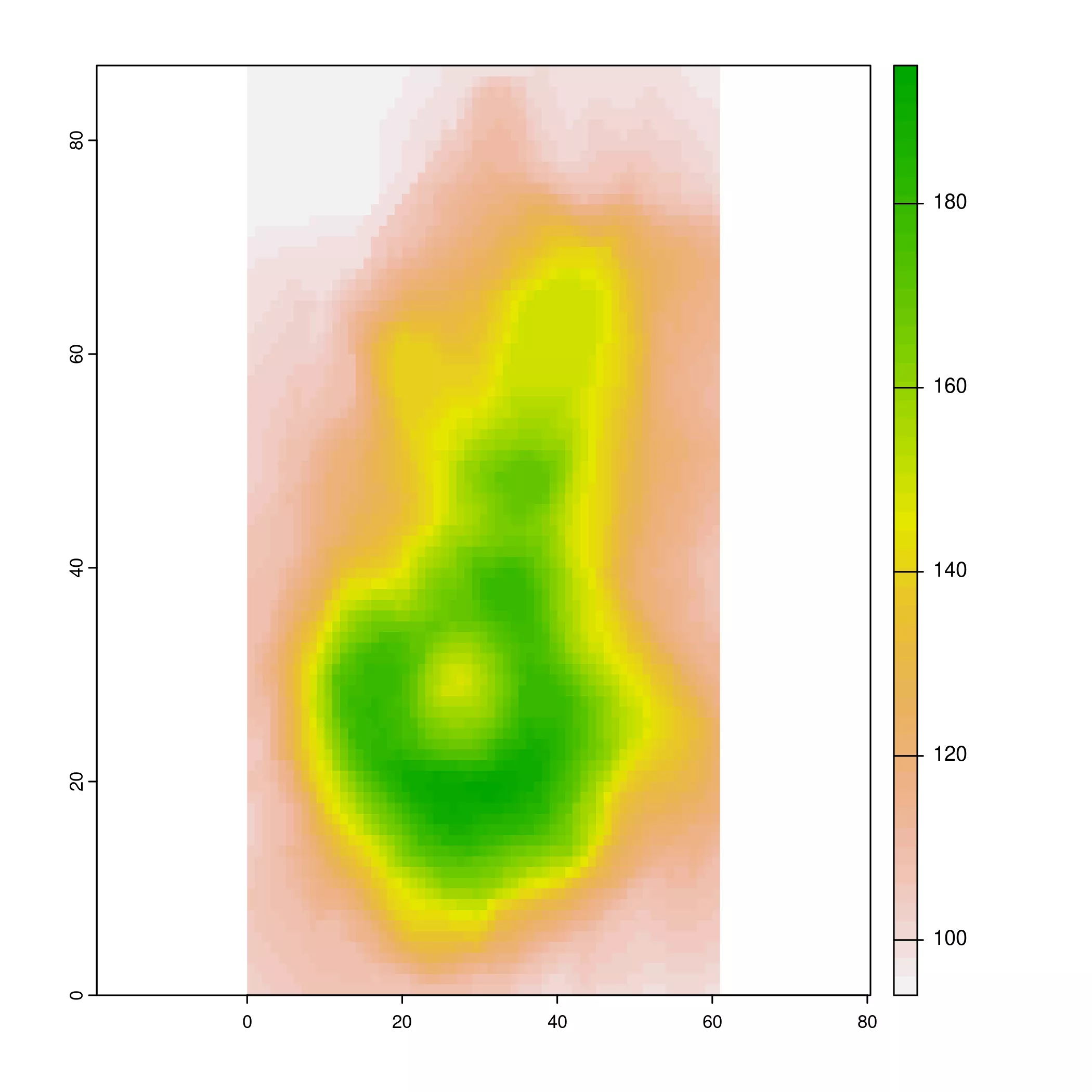
volcano_rast_ok
#> class       : SpatRaster
#> dimensions  : 87, 61, 1  (nrow, ncol, nlyr)
#> resolution  : 1, 1  (x, y)
#> extent      : 0, 61, 0, 87  (xmin, xmax, ymin, ymax)
#> coord. ref. :
#> source      : memory
#> name        : lyr.1
#> min value   :    94
#> max value   :   195
Nice! Now we have a raster of volcano, but still without geotagged
information. Thanks to this article by Tomislav Hengl
(@tom_hengl) we can check the basic geographic
parameters of volcano (see Volcano
Maungawhau), which are:
- CRS: EPSG:27200
- xllcorner: 2667400
- yllcorner: 6478700
- cellsize: 10 m
- ncols: 61
- nrows: 87
And we can translate that easily to an empty SpatRaster:
# Extra length for proper handling extent
xrange <- range(seq(from = 2667400, length.out = 62, by = 10))
yrange <- range(seq(from = 6478700, length.out = 88, by = 10))

template <- rast(
  crs = "EPSG:27200",
  xmin = xrange[1],
  xmax = xrange[2],
  ymin = yrange[1],
  ymax = yrange[2],
  resolution = 10
)
template
#> class       : SpatRaster
#> dimensions  : 87, 61, 1  (nrow, ncol, nlyr)
#> resolution  : 10, 10  (x, y)
#> extent      : 2667400, 2668010, 6478700, 6479570  (xmin, xmax, ymin, ymax)
#> coord. ref. : NZGD49 / New Zealand Map Grid (EPSG:27200)
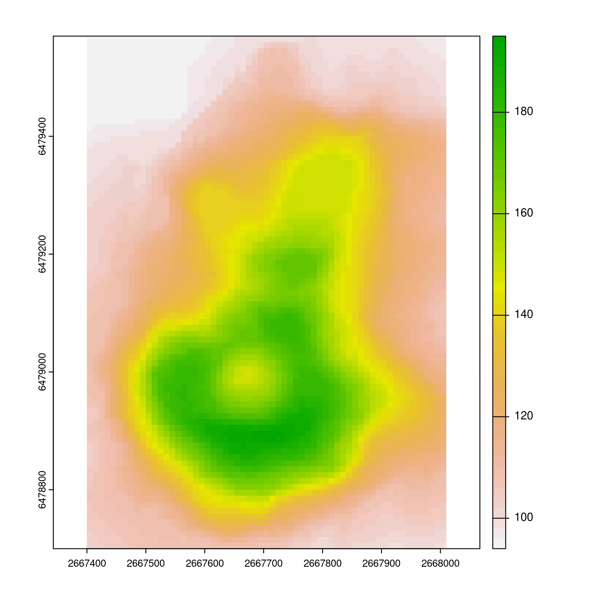
So now we only need to transfer the values from volcano_rast_ok to our
template:
# Use tidyterra to pull the values of one raster
# and create a new layer

volcano2 <- template %>%
  mutate(elevation = pull(volcano_rast_ok, lyr.1)) %>%
  select(elevation)

volcano2
#> class       : SpatRaster
#> dimensions  : 87, 61, 1  (nrow, ncol, nlyr)
#> resolution  : 10, 10  (x, y)
#> extent      : 2667400, 2668010, 6478700, 6479570  (xmin, xmax, ymin, ymax)
#> coord. ref. : NZGD49 / New Zealand Map Grid (EPSG:27200)
#> source      : memory
#> name        : elevation
#> min value   :        94
#> max value   :       195

terra::plot(volcano2)
# And plot it
ggtile +
  geom_spatraster(data = volcano2) +
  scale_fill_terrain_c(alpha = 0.75)
An Easter egg
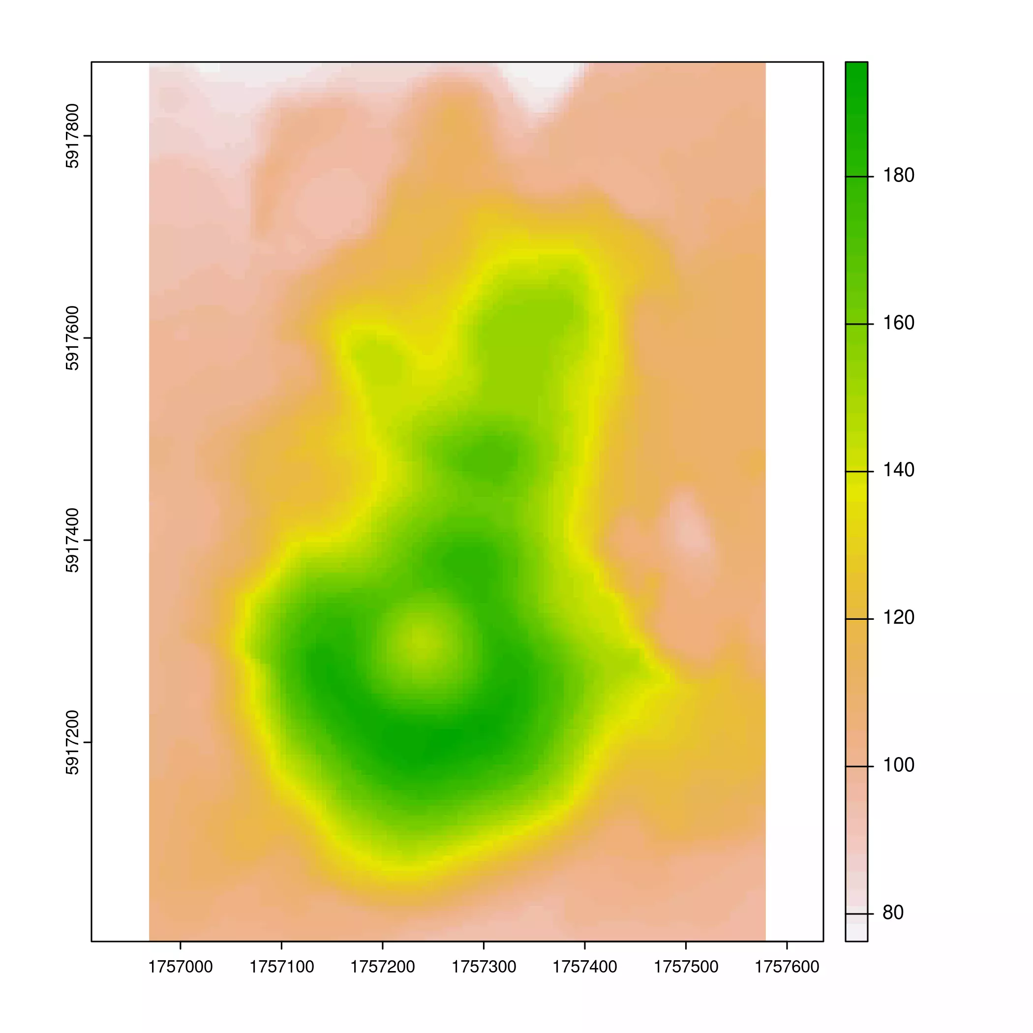
The volcano dataset may not be completely up to date. As a complement,
tidyterra includes a .tif file with the same dimensions as our volcano2
raster, but with the topographic values extracted from Auckland LiDAR 1m DEM
(2013) and
resampled to a resolution of 5x5 meters, for package size optimization. See here
how to load it and check the plotting possibilities of tidyterra:
# Load out Easter Egg

volcano2_easter <- rast(system.file("extdata/volcano2.tif",
  package = "tidyterra"
))

volcano2_easter
#> class       : SpatRaster
#> dimensions  : 174, 122, 1  (nrow, ncol, nlyr)
#> resolution  : 5, 5  (x, y)
#> extent      : 1756969, 1757579, 5917003, 5917873  (xmin, xmax, ymin, ymax)
#> coord. ref. : NZGD2000 / New Zealand Transverse Mercator 2000 (EPSG:2193)
#> source      : volcano2.tif
#> name        : elevation
#> min value   :  76.26222
#> max value   :  195.5542
terra::plot(volcano2_easter)
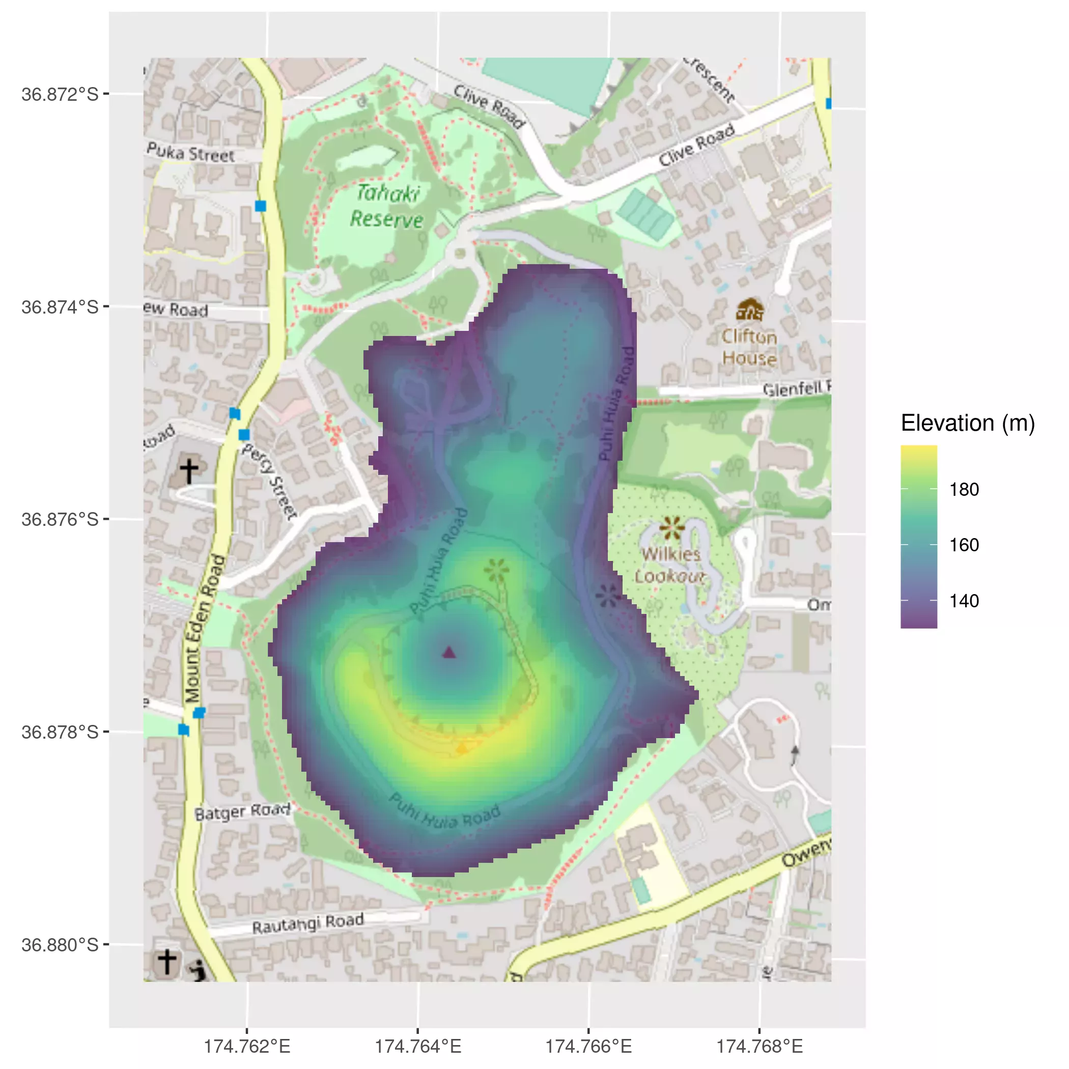
# Only altitudes of more than 130m

volcano_filter <- volcano2_easter %>%
  filter(elevation > 130)


ggtile +
  geom_spatraster(data = volcano_filter) +
  scale_fill_viridis_c(na.value = NA, alpha = 0.7) +
  labs(fill = "Elevation (m)")
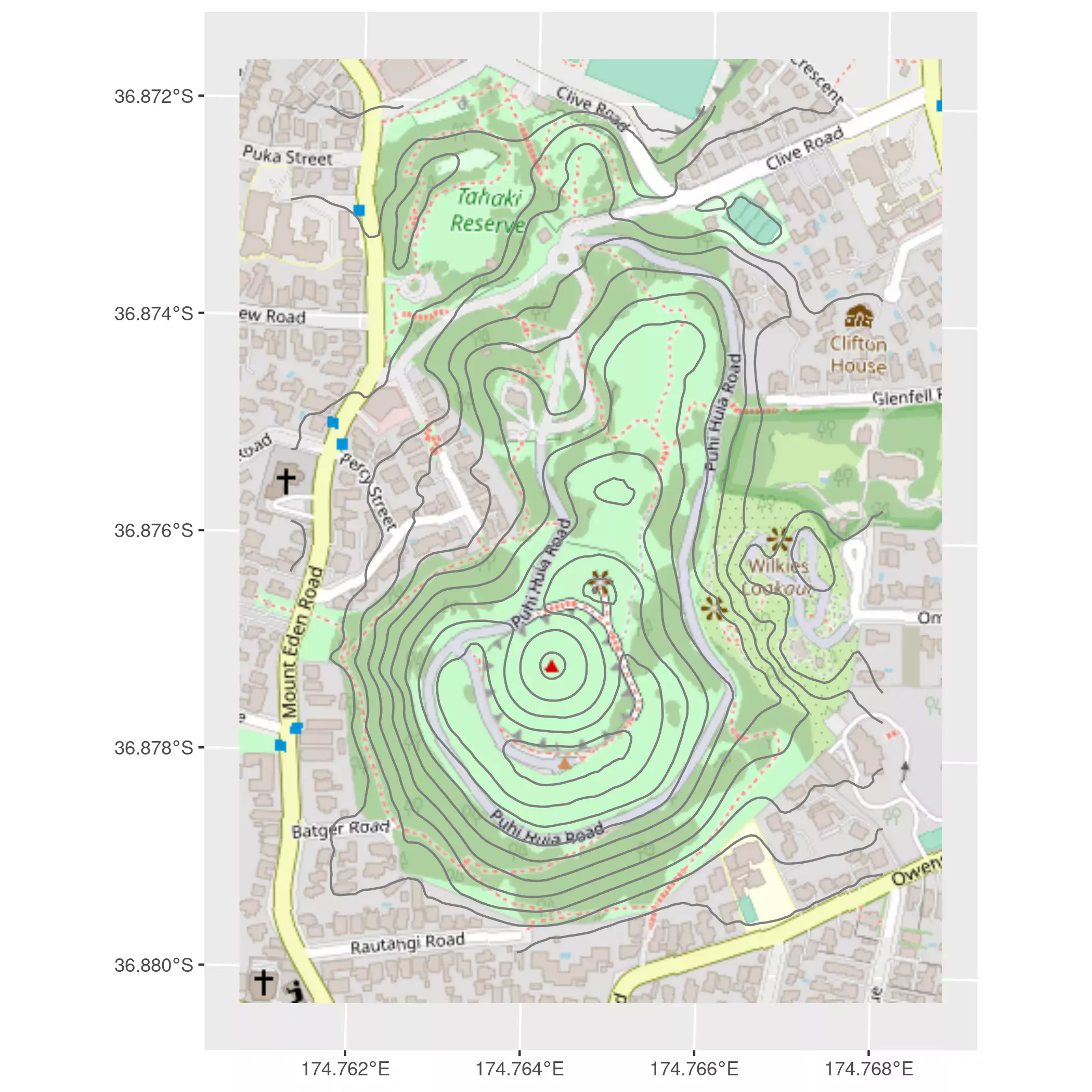
# Contour lines

ggtile +
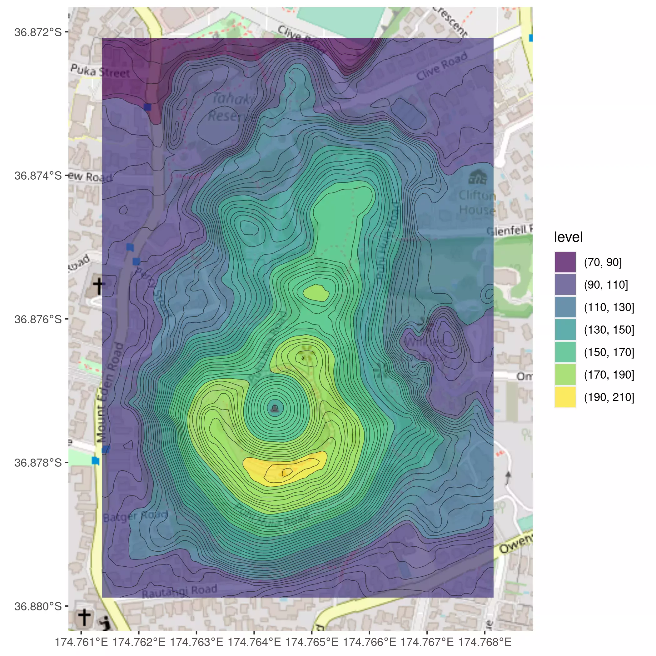
  geom_spatraster_contour(data = volcano2_easter, binwidth = 10)
# Contour lines + contour polygons

ggtile +
  geom_spatraster_contour_filled(
    data = volcano2_easter,
    breaks = seq(70, 210, 20),
    alpha = 0.7
  ) +
  geom_spatraster_contour(
    data = volcano2_easter, binwidth = 2.5,
    alpha = 0.7, size = .2, color = "grey10"
  ) +
  coord_sf(expand = FALSE)