This vignette introduces the main data sets and functions in igoR with visual examples.
The examples build on analyses from Pevehouse et al. (2020). For more information about the IGO data sets and additional downloads, see Intergovernmental Organizations (version 3).
The original dyad-year data set is not included because of its size (about 500 MB in Stata .dta format). The igo_dyadic() function derives comparable joint membership results from the included data.
Definitions
From Pevehouse et al. (2019):
What is an IGO?
The original data set defines an intergovernmental organization (IGO) using the following criteria:
- An IGO must consist of at least three members of the Correlates of War state system.
- An IGO must hold regular plenary sessions at least once every ten years.
- An IGO must possess a permanent secretariat and corresponding headquarters.
When does an IGO begin?
The data set begins coding an IGO in the first year the organization functions. In some cases, individual members are recorded by year of accession or signature.
When does an IGO cease to exist?
Version 3.0 of the IGO data set uses the following criteria:
- An organization is considered terminated when its description includes one of the following terms:
replaced,succeeded,superseded,integrated,mergedordies.
Analysis
This section reproduces selected analyses based on figures in Pevehouse et al. (2020).
Initial setup
First, create a custom ggplot2::theme() object named theme_igor. All figures in this vignette use this theme.
theme_igor <- theme(
  axis.title = element_blank(),
  axis.line.x.bottom = element_line("black"),
  axis.line.y.left = element_line("black"),
  axis.text = element_text(color = "black", family = "sans"),
  axis.text.y.left = element_text(angle = 90, hjust = 0.5),
  legend.position = "bottom",
  legend.title = element_blank(),
  legend.key = element_blank(),
  legend.key.width = unit(2, "cm"),
  legend.text = element_text(family = "sans", size = 11.5),
  legend.box.background = element_rect(color = "black", linewidth = 1),
  legend.spacing = unit(1.2 / 100, "npc"),
  plot.background = element_rect("grey90"),
  plot.margin = unit(rep(0.5, 4), "cm"),
  panel.background = element_rect("white"),
  panel.grid = element_blank(),
  panel.border = element_rect(fill = NA, colour = "grey90"),
  panel.grid.major.y = element_line("grey90")
)
IGOs overview
The following code counts IGOs and states in the Correlates of War (COW) system by year. The data cover 1816 to 2014.
# Summarize values by year.
igos_by_year <- igo_year_format3 %>%
  group_by(year) %>%
  summarise(value = n(), .groups = "keep") %>%
  mutate(variable = "Total IGOs")

countries_by_year <- state_year_format3 %>%
  group_by(year) %>%
  summarise(value = n(), .groups = "keep") %>%
  mutate(variable = "Number of COW states")

all_by_year <- igos_by_year %>%
  bind_rows(countries_by_year) %>%
  # Label the plot.
  mutate(
    variable = factor(
      variable,
      levels = c("Total IGOs", "Number of COW states")
    )
  )

# Plot the results.
ggplot(all_by_year, aes(x = year, y = value)) +
  geom_line(color = "black", aes(linetype = variable)) +
  scale_x_continuous(limits = c(1800, 2014)) +
  scale_linetype_manual(values = c("solid", "dashed")) +
  geom_vline(xintercept = c(1945, 1989)) +
  ylim(0, 400) +
  theme_igor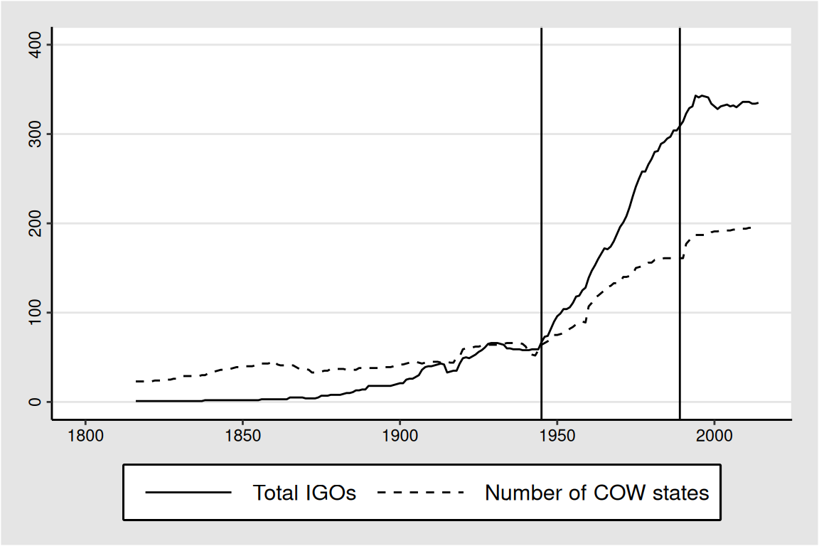
IGO starts and endings
This plot shows how many IGOs started or ended in each year.
# Summarize IGO starts and endings by year.

df <- igo_search()

births <- df %>%
  mutate(year = sdate) %>%
  group_by(year) %>%
  summarise(value = n(), .groups = "keep") %>%
  mutate(variable = "IGO births")

deads <- df %>%
  mutate(year = deaddate) %>%
  group_by(year) %>%
  summarise(value = n(), .groups = "keep") %>%
  mutate(variable = "IGO deaths")

births_and_deads <- births %>%
  bind_rows(deads) %>%
  filter(!is.na(year))

# Plot the results.
ggplot(births_and_deads, aes(x = year, y = value)) +
  geom_line(color = "black", aes(linetype = variable)) +
  scale_linetype_manual(values = c("solid", "dashed")) +
  scale_x_continuous(
    limits = c(1815, 2015),
    breaks = seq(1815, 2015, by = 25)
  ) +
  ylim(0, 15) +
  theme_igor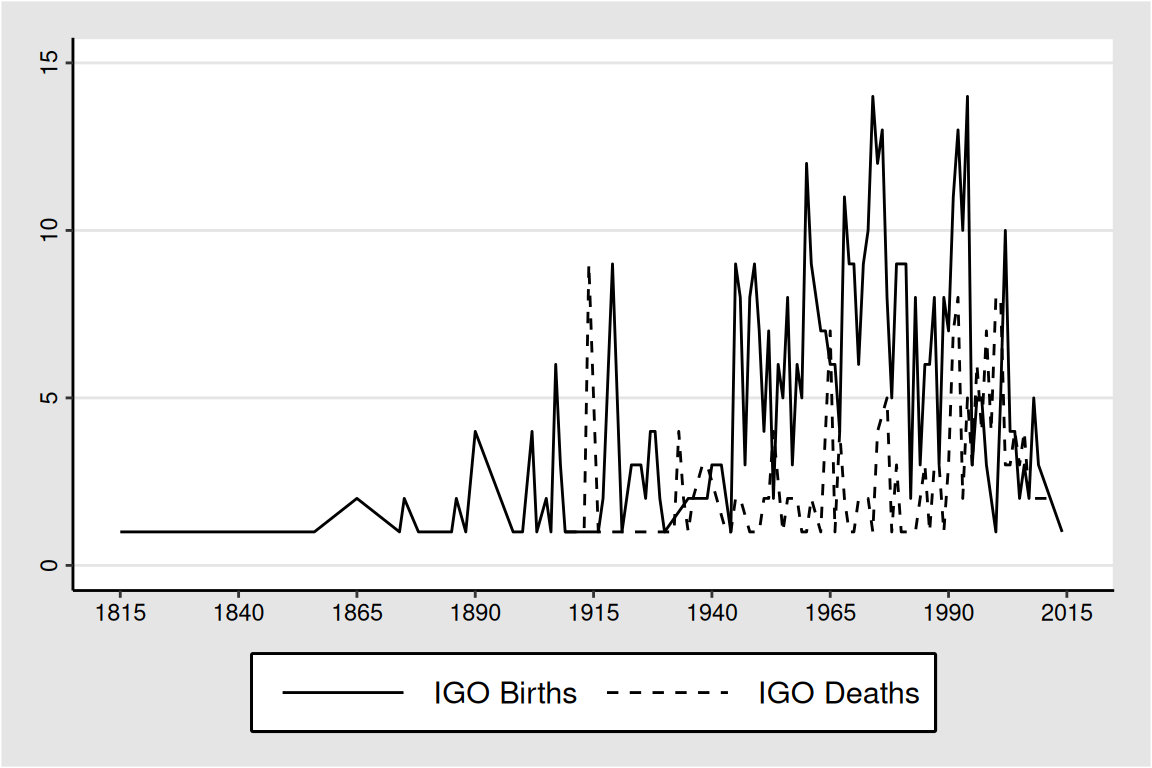
IGOs across regions
This plot shows the number of IGOs by region. The regional definitions are based on Pevehouse et al. (2020) and the complementary replication data set (PRIO 2020).
IGOs across regions: codes
# Cross-regional and universal codes are not included.

asia <- c(
  550,
  560,
  570,
  580,
  590,
  600,
  610,
  640,
  650,
  660,
  670,
  725,
  750,
  825,
  1030,
  1345,
  1400,
  1530,
  1532,
  2300,
  2770,
  3185,
  3330,
  3560,
  3930,
  4115,
  4150,
  4160,
  4170,
  4190,
  4200,
  4220,
  4265,
  4440
)

middle_east <- c(
  370,
  380,
  390,
  400,
  410,
  420,
  430,
  440,
  450,
  460,
  470,
  490,
  500,
  510,
  520,
  1110,
  1410,
  1990,
  2000,
  2220,
  3450,
  3800,
  4140,
  4270,
  4380
)

europe <- c(
  20,
  300,
  780,
  800,
  832,
  840,
  860,
  1020,
  1050,
  1070,
  1080,
  1125,
  1140,
  1390,
  1420,
  1440,
  1563,
  1565,
  1580,
  1585,
  1590,
  1600,
  1610,
  1620,
  1630,
  1640,
  1645,
  1653,
  1660,
  1670,
  1675,
  1680,
  1690,
  1700,
  1710,
  1715,
  1720,
  1730,
  1740,
  1750,
  1760,
  1770,
  1780,
  1790,
  1800,
  1810,
  1820,
  1830,
  1930,
  1970,
  1980,
  2310,
  2325,
  2345,
  2440,
  2450,
  2550,
  2575,
  2610,
  2650,
  2705,
  2890,
  2972,
  3010,
  3095,
  3230,
  3290,
  3360,
  3485,
  3505,
  3585,
  3590,
  3600,
  3610,
  3620,
  3630,
  3640,
  3650,
  3655,
  3660,
  3665,
  3762,
  3810,
  3855,
  3860,
  3910,
  4000,
  4350,
  4450,
  4460,
  4510,
  4520,
  4540
)

africa <- c(
  30,
  40,
  50,
  60,
  80,
  90,
  100,
  110,
  115,
  120,
  125,
  130,
  140,
  150,
  155,
  160,
  170,
  180,
  190,
  200,
  210,
  225,
  240,
  250,
  260,
  280,
  290,
  690,
  700,
  710,
  940,
  1060,
  1150,
  1170,
  1260,
  1290,
  1310,
  1320,
  1330,
  1340,
  1355,
  1430,
  1450,
  1460,
  1470,
  1475,
  1480,
  1500,
  1510,
  1520,
  1870,
  2080,
  2090,
  2230,
  2330,
  2795,
  3300,
  3310,
  3470,
  3480,
  3510,
  3520,
  3570,
  3740,
  3760,
  3761,
  3790,
  3820,
  3875,
  3905,
  3970,
  4010,
  4030,
  4050,
  4055,
  4080,
  4110,
  4120,
  4130,
  4230,
  4240,
  4250,
  4251,
  4340,
  4365,
  4480,
  4485,
  4490,
  4500,
  4501,
  4503
)

americas <- c(
  310,
  320,
  330,
  340,
  720,
  760,
  815,
  875,
  880,
  890,
  900,
  910,
  912,
  913,
  920,
  950,
  970,
  980,
  990,
  1000,
  1010,
  1095,
  1130,
  1486,
  1489,
  1490,
  1860,
  1890,
  1920,
  1950,
  2070,
  2110,
  2120,
  2130,
  2140,
  2150,
  2160,
  2170,
  2175,
  2180,
  2190,
  2200,
  2203,
  2206,
  2210,
  2260,
  2340,
  2490,
  2560,
  2980,
  3060,
  3340,
  3370,
  3380,
  3390,
  3400,
  3410,
  3420,
  3428,
  3430,
  3670,
  3680,
  3812,
  3830,
  3880,
  3890,
  3900,
  3925,
  3980,
  4070,
  4100,
  4260,
  4280,
  4370
)
# `africa`, `americas`, `asia`, `europe` and `middle_east` were created in the
# previous chunk, which is collapsed for readability.

regions <- igo_search() %>%
  mutate(
    region = case_when(
      ionum %in% africa ~ "Africa",
      ionum %in% americas ~ "Americas",
      ionum %in% asia ~ "Asia",
      ionum %in% europe ~ "Europe",
      ionum %in% middle_east ~ "Middle East",
      TRUE ~ NA
    )
  ) %>%
  select(ioname, region)
The next step joins the region classifications to the IGO-year data and counts IGOs by region.
# The `regions` data set was created in the previous chunk.

# Select all IGOs.
alligos <- igo_year_format3 %>%
  select(ioname, year)

regionsum <- alligos %>%
  left_join(regions) %>%
  group_by(year, region) %>%
  summarise(value = n(), .groups = "keep") %>%
  filter(!is.na(region)) %>%
  # Prepare for plotting.
  mutate(
    region = factor(
      region,
      levels = c(
        "Asia",
        "Europe",
        "Africa",
        "Americas",
        "Middle East"
      )
    )
  )

# Plot the results.
ggplot(regionsum, aes(x = year, y = value)) +
  geom_line(color = "black", aes(linetype = region)) +
  scale_linetype_manual(
    values = c("solid", "dashed", "dotted", "dotdash", "longdash")
  ) +
  guides(linetype = guide_legend(ncol = 2, byrow = TRUE)) +
  ylim(0, 80) +
  scale_x_continuous(
    limits = c(1815, 2015),
    breaks = seq(1815, 2015, by = 25)
  ) +
  theme_igor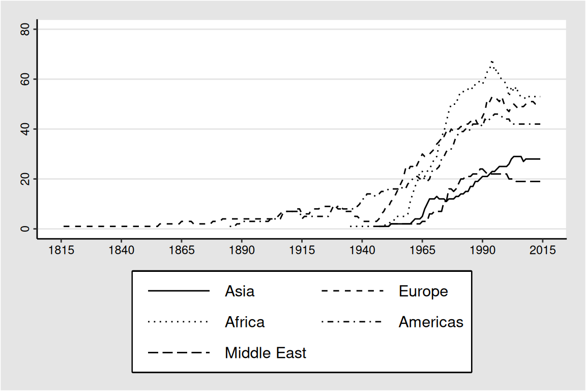
Selected states in Asia
This plot shows the number of full IGO memberships for five states in Asia: India, China, Pakistan, Indonesia and Bangladesh.
asia5_cntries <- c("China", "India", "Pakistan", "Indonesia", "Bangladesh")

# Use five states in Asia.
asia5_igos <- igo_state_membership(
  state = asia5_cntries,
  year = 1865:2014,
  status = "Full Membership"
)

asia5 <- asia5_igos %>%
  group_by(statenme, year) %>%
  summarise(values = n(), .groups = "keep") %>%
  mutate(statenme = factor(statenme, levels = asia5_cntries))

# Plot the results.
ggplot(asia5, aes(x = year, y = values)) +
  geom_line(color = "black", aes(linetype = statenme)) +
  scale_linetype_manual(
    values = c("solid", "dashed", "dotted", "dotdash", "longdash")
  ) +
  guides(linetype = guide_legend(ncol = 3, byrow = TRUE)) +
  theme(
    axis.title.y.left = element_text(
      family = "sans",
      size = 12,
      margin = margin(r = 6)
    )
  ) +
  scale_x_continuous(
    limits = c(1865, 2015),
    breaks = seq(1865, 2015, by = 25)
  ) +
  scale_y_continuous(
    "Number of memberships",
    breaks = seq(0, 100, 20),
    limits = c(0, 100)
  ) +
  theme_igor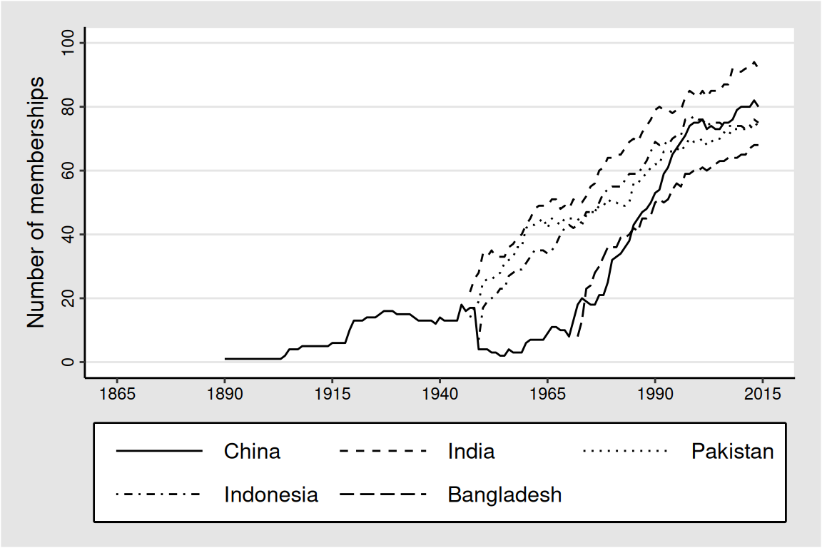
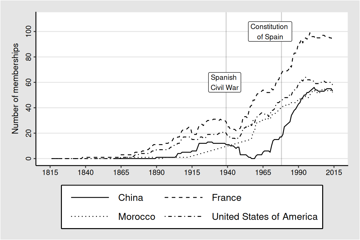
Joint memberships
The final plot counts full joint memberships in dyad-year data for Spain and four selected states.
selected_countries <- c("France", "Morocco", "China", "USA")

spain_selected <- igo_dyadic("Spain", selected_countries)

# Compute the number of full joint memberships.
spain_selected <- spain_selected %>%
  rowwise() %>%
  mutate(values = sum(c_across(aaaid:wassen) == 1))

# Plot the results.
ggplot(spain_selected, aes(x = year, y = values)) +
  geom_line(color = "black", aes(linetype = statenme2)) +
  scale_linetype_manual(values = c("solid", "dashed", "dotted", "dotdash")) +
  guides(linetype = guide_legend(ncol = 2, byrow = TRUE)) +
  theme(
    axis.title.y.left = element_text(
      family = "sans",
      size = 10,
      margin = margin(r = 6)
    )
  ) +
  scale_x_continuous(
    limits = c(1815, 2015),
    breaks = seq(1815, 2015, by = 25)
  ) +
  scale_y_continuous(
    "Number of memberships",
    breaks = seq(0, 110, 20),
    limits = c(0, 110)
  ) +
  theme_igor +
  geom_vline(xintercept = 1939, alpha = 0.2) +
  annotate("label", x = 1938, y = 60, size = 3, label = "Spanish \nCivil War") +
  geom_vline(xintercept = 1978, alpha = 0.2) +
  annotate(
    "label",
    x = 1970,
    y = 100,
    size = 3,
    label = "Constitution \nof Spain"
  )