Maps can show how membership in intergovernmental organizations (IGOs) changes across states and time.
This vignette presents geospatial visualizations using the IGO data sets (Pevehouse et al. 2020) included in igoR. It uses these packages for geospatial data:
- giscoR package for extracting country geometries.
- ggplot2 package for plotting.
- sf package for working with spatial features.
The countrycode package is useful for translating country names and codes across schemes such as Correlates of War (COW), ISO3, NUTS and FIPS.
library(igoR)

# Helper packages.
library(dplyr)
library(ggplot2)
library(countrycode)

# Geospatial packages.
library(giscoR)
library(sf)
Evolution of UN membership
The following map shows the evolution of United Nations membership. First, extract the membership data.
# Extract shapes.
world <- gisco_get_countries()

# Extract three years. Some COW codes do not have ISO equivalents.
un_all <- igo_members("UN", c(1950, 1980, 2010), status = "Full Membership") %>%
  # Add the ISO3 code.
  mutate(ISO3_CODE = countrycode(ccode, "cown", "iso3c", warn = FALSE)) %>%
  select(year, orgname, ISO3_CODE, category)

# Build an auxiliary data frame to collect every ISO3-year pair.
base_df <- expand.grid(
  ISO3_CODE = unique(world$ISO3_CODE),
  year = unique(un_all$year),
  stringsAsFactors = FALSE
) %>%
  as_tibble()

# Merge everything with the spatial object.
un_all_sf <- world %>%
  # Expand to all cases.
  left_join(base_df, by = "ISO3_CODE") %>%
  # Add information.
  left_join(un_all, by = c("ISO3_CODE", "year"))
The map is approximate because the base geometries represent modern states. Historical states such as Czechoslovakia, East Germany and West Germany are not included.
The data are now ready to plot with ggplot2.
ggplot(un_all_sf) +
  geom_sf(aes(fill = category), color = NA, show.legend = FALSE) +
  # Robinson
  coord_sf(crs = "ESRI:54030") +
  facet_wrap(~year, ncol = 1, strip.position = "left") +
  scale_fill_manual(
    values = c("Full Membership" = "#74A9CF"),
    na.value = "#E0E0E0",
  ) +
  labs(
    title = "UN members",
    caption = gisco_attributions(),
  ) +
  theme_minimal() +
  theme(
    plot.caption = element_text(face = "italic", hjust = 0.15),
    axis.line = element_blank(),
    axis.text = element_blank()
  )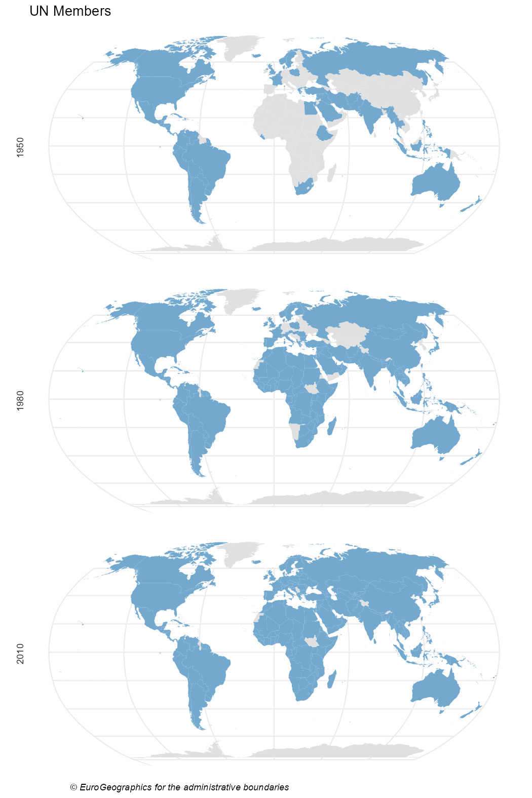
Figure 1: UN members (1950, 1980, 2010)
Joint memberships with Australia
Joint memberships are useful for identifying regional patterns. The following code maps the number of IGOs in which each state and Australia were both full members in 2014.
# Count full joint memberships in 2014.
# Find states in the state system in 2014.
states2014 <- states2016 %>%
  filter(styear <= 2014 & endyear >= 2014)

# Find joint memberships with Australia.
shared <- igo_dyadic("AUL", as.character(states2014$statenme), year = 2014) %>%
  rowwise() %>%
  mutate(shared = sum(c_across(aaaid:wassen) == 1)) %>%
  mutate(ISO3_CODE = countrycode(ccode2, "cown", "iso3c", warn = FALSE)) %>%
  select(ISO3_CODE, shared)

# Merge with the map.
sharedmap <- world %>%
  left_join(shared, by = "ISO3_CODE") %>%
  select(ISO3_CODE, shared)

# Plot with a custom palette.
pal <- hcl.colors(10, palette = "Lajolla")

# Plot the results.
ggplot(sharedmap) +
  geom_sf(aes(fill = shared), color = NA) +
  # Highlight Australia.
  geom_sf(
    data = sharedmap %>% filter(ISO3_CODE == "AUS"),
    fill = "black",
    color = NA,
  ) +
  # Robinson
  coord_sf(crs = "ESRI:54030") +
  scale_fill_gradientn(colours = pal, n.breaks = 10) +
  guides(fill = guide_legend(nrow = 1)) +
  labs(
    title = "Shared full memberships with Australia (2014)",
    fill = "Number of joint memberships",
    caption = gisco_attributions()
  ) +
  theme_minimal() +
  theme(
    plot.title = element_text(face = "bold", hjust = 0.5),
    plot.caption = element_text(face = "italic", size = 7, hjust = 0.15),
    axis.line = element_blank(),
    axis.text = element_blank(),
    legend.title = element_text(size = 7),
    legend.text = element_text(size = 8),
    legend.position = "bottom",
    legend.direction = "horizontal",
    legend.title.position = "top",
    legend.text.position = "bottom",
    legend.key.width = unit(1.5, "lines"),
    legend.key.height = unit(0.5, "lines")
  )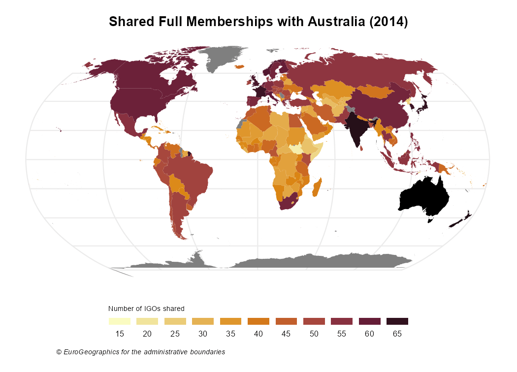
Figure 2: Full joint memberships with Australia (2014)
Joint memberships across North America
The following map shows how the number of full joint memberships among North American states changed from 1930 to 2010 at ten-year intervals.
# Select years.
years <- seq(1930, 2010, 10)

# Find joint memberships.
cntries <- c("USA", "CAN", "MEX")
all <- igo_dyadic(cntries, cntries, years) %>%
  rowwise() %>%
  mutate(value = sum(c_across(aaaid:wassen) == 1)) %>%
  mutate(ISO3_CODE = countrycode(ccode1, "cown", "iso3c")) %>%
  select(ISO3_CODE, year, value)

# Get shapes for the map.
countries_sf <- gisco_get_countries(country = c("USA", "MEX", "CAN")) %>%
  left_join(all, by = "ISO3_CODE")

# Plot the map.
ggplot(countries_sf) +
  geom_sf(aes(fill = value), color = NA) +
  coord_sf(crs = 9311, xlim = c(-3200000, 3333018)) +
  facet_wrap(~year, ncol = 3) +
  scale_fill_gradientn(
    colors = hcl.colors(10, "YlGn", rev = TRUE),
    breaks = seq(0, 100, 5)
  ) +
  guides(fill = guide_legend(reverse = TRUE)) +
  labs(
    title = "Shared full memberships in North America",
    subtitle = "(1930-2010)",
    fill = "Joint memberships",
    caption = gisco_attributions()
  ) +
  theme_minimal() +
  theme(
    panel.grid = element_blank(),
    axis.line = element_blank(),
    axis.text = element_blank(),
    strip.background = element_rect(fill = "grey90", colour = NA)
  )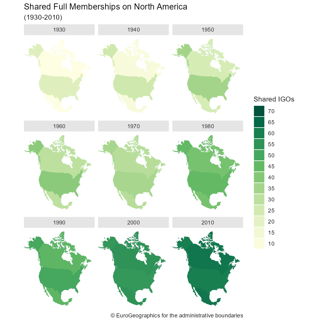
Figure 3: Full joint memberships in North America (1930-2010)