Geotag an image and return a SpatRaster based on coordinates from a
supported spatial input class.
rasterpic_img() is an S3 generic. See S3 methods for supported input
classes.
Usage
rasterpic_img(
  x,
  img,
  halign = 0.5,
  valign = 0.5,
  expand = 0,
  crop = FALSE,
  ...
)

# S3 method for class 'sf'
rasterpic_img(
  x,
  img,
  halign = 0.5,
  valign = 0.5,
  expand = 0,
  crop = FALSE,
  ...,
  mask = FALSE,
  inverse = FALSE
)

# S3 method for class 'sfc'
rasterpic_img(
  x,
  img,
  halign = 0.5,
  valign = 0.5,
  expand = 0,
  crop = FALSE,
  ...,
  mask = FALSE,
  inverse = FALSE
)

# S3 method for class 'sfg'
rasterpic_img(
  x,
  img,
  halign = 0.5,
  valign = 0.5,
  expand = 0,
  crop = FALSE,
  ...,
  mask = FALSE,
  inverse = FALSE,
  crs = NULL
)

# S3 method for class 'stars'
rasterpic_img(
  x,
  img,
  halign = 0.5,
  valign = 0.5,
  expand = 0,
  crop = FALSE,
  ...
)

# S3 method for class 'bbox'
rasterpic_img(
  x,
  img,
  halign = 0.5,
  valign = 0.5,
  expand = 0,
  crop = FALSE,
  ...,
  crs = NULL
)

# S3 method for class 'numeric'
rasterpic_img(
  x,
  img,
  halign = 0.5,
  valign = 0.5,
  expand = 0,
  crop = FALSE,
  ...,
  crs = NULL
)

# S3 method for class 'SpatRaster'
rasterpic_img(
  x,
  img,
  halign = 0.5,
  valign = 0.5,
  expand = 0,
  crop = FALSE,
  ...
)

# S3 method for class 'SpatVector'
rasterpic_img(
  x,
  img,
  halign = 0.5,
  valign = 0.5,
  expand = 0,
  crop = FALSE,
  ...,
  mask = FALSE,
  inverse = FALSE
)

# S3 method for class 'SpatExtent'
rasterpic_img(
  x,
  img,
  halign = 0.5,
  valign = 0.5,
  expand = 0,
  crop = FALSE,
  ...,
  crs = NULL
)
Arguments
- x
An R object. See S3 methods for supported classes.
- img
An image to geotag. It can be a local file or a URL, for example
"https://i.imgur.com/6yHmlwT.jpeg". Accepted file extensions arepng,jpg,jpeg,tifandtiff.- halign
A number between
0and1giving the horizontal alignment ofimgrelative tox.0alignsimgwith the left edge ofx,1aligns it with the right edge and0.5centers it horizontally.- valign
A number between
0and1giving the vertical alignment ofimgrelative tox.0alignsimgwith the bottom edge ofx,1aligns it with the top edge and0.5centers it vertically.- expand
An expansion factor of the bounding box of
x.0means that no expansion is added,1means that the bounding box is expanded to double the original size. See Details.- crop
Logical. Should the raster be cropped to the (expanded) bounding box of
x? See Details.- ...
Further arguments passed to methods.
- mask
Logical, for vector methods. Should the raster be masked to the shape of
x? See Details.- inverse
Logical. Only used when
mask = TRUE. IfTRUE, areas of the raster covered byxare masked.- crs
Character string describing a CRS. This parameter only applies when
xis aSpatExtent,sfg,bboxor a numeric coordinate vector. See the CRS section.
Value
A SpatRaster object (see terra::rast()) where each layer corresponds to
a color channel of img:
If
imghas at least 3 layers, the result records layers 1 to 3 as the red, green and blue channels with names"r","g"and"b"andalphaif applicable.If
imgalready has an RGB specification (this may be the case fortif/tifffiles), the result keeps that specification.
The resulting SpatRaster will have an RGB specification as explained in
terra::RGB().
Details
vignette("rasterpic", package = "rasterpic") explains the effect of
parameters halign, valign, expand, crop and mask with examples.
S3 methods
rasterpic supports these spatial input classes:
sf classes:
sf,sfc,sfgandbbox.terra classes:
SpatRaster,SpatVectorandSpatExtent.stars class:
stars.A numeric coordinate vector of the form
c(xmin, ymin, xmax, ymax).
Other packages can provide methods for additional spatial classes.
Methods for extent-like inputs use the object extent. Methods for vector inputs can also mask the image to the object shape.
CRS
This function preserves the CRS of x when applicable. For optimal results,
do not use geographic coordinates (longitude/latitude).
crs can be in WKT format, as an "authority:number" code such as
"EPSG:4326" or as a PROJ-string such as "+proj=utm +zone=12". It can also
be retrieved with:
See the Value and Notes sections in terra::crs().
See also
vignette("rasterpic", package = "rasterpic") for examples.
From sf:
vignette("sf1", package = "sf")to understand how sf organizes R objects.
From stars:
From terra:
For plotting:
Examples
# \donttest{
library(sf)
#> Linking to GEOS 3.12.1, GDAL 3.8.4, PROJ 9.4.0; sf_use_s2() is TRUE
library(terra)
library(ggplot2)
library(tidyterra)
#>
#> Attaching package: ‘tidyterra’
#> The following object is masked from ‘package:stats’:
#>
#> filter
x_path <- system.file("gpkg/UK.gpkg", package = "rasterpic")
x <- st_read(x_path, quiet = TRUE)
img <- system.file("img/vertical.png", package = "rasterpic")
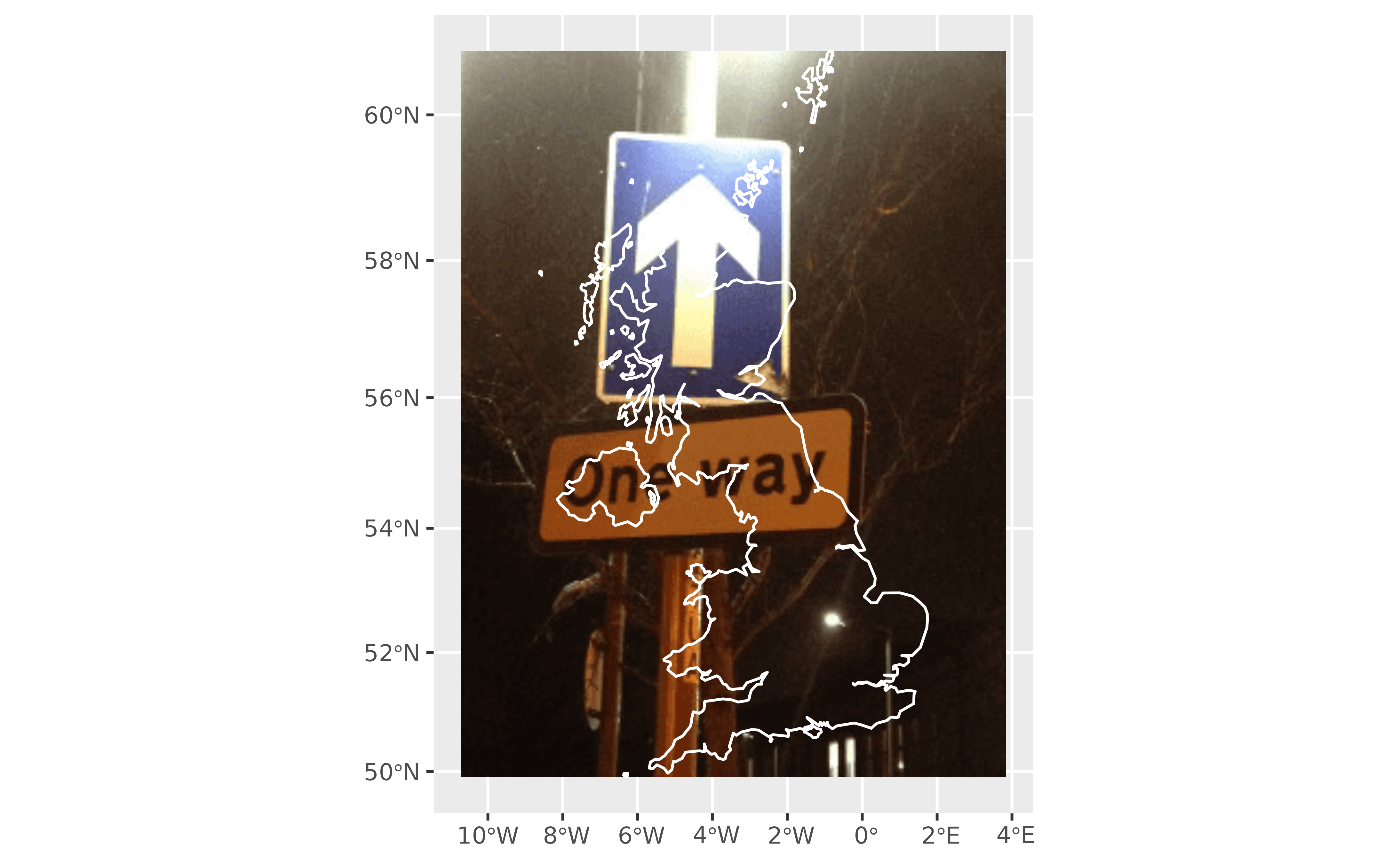
# Use the default configuration.
ex1 <- rasterpic_img(x, img)
ex1
#> class : SpatRaster
#> size : 333, 250, 3 (nrow, ncol, nlyr)
#> resolution : 6484.467, 6484.467 (x, y)
#> extent : -1193414, 427703.2, 6430573, 8589900 (xmin, xmax, ymin, ymax)
#> coord. ref. : WGS 84 / Pseudo-Mercator (EPSG:3857)
#> source(s) : memory
#> colors rgb : 1, 2, 3
#> names : r, g, b
#> min values : 15, 8, 4
#> max values : 254, 255, 254
autoplot(ex1) +
geom_sf(data = x, fill = NA, color = "white", linewidth = 0.5)
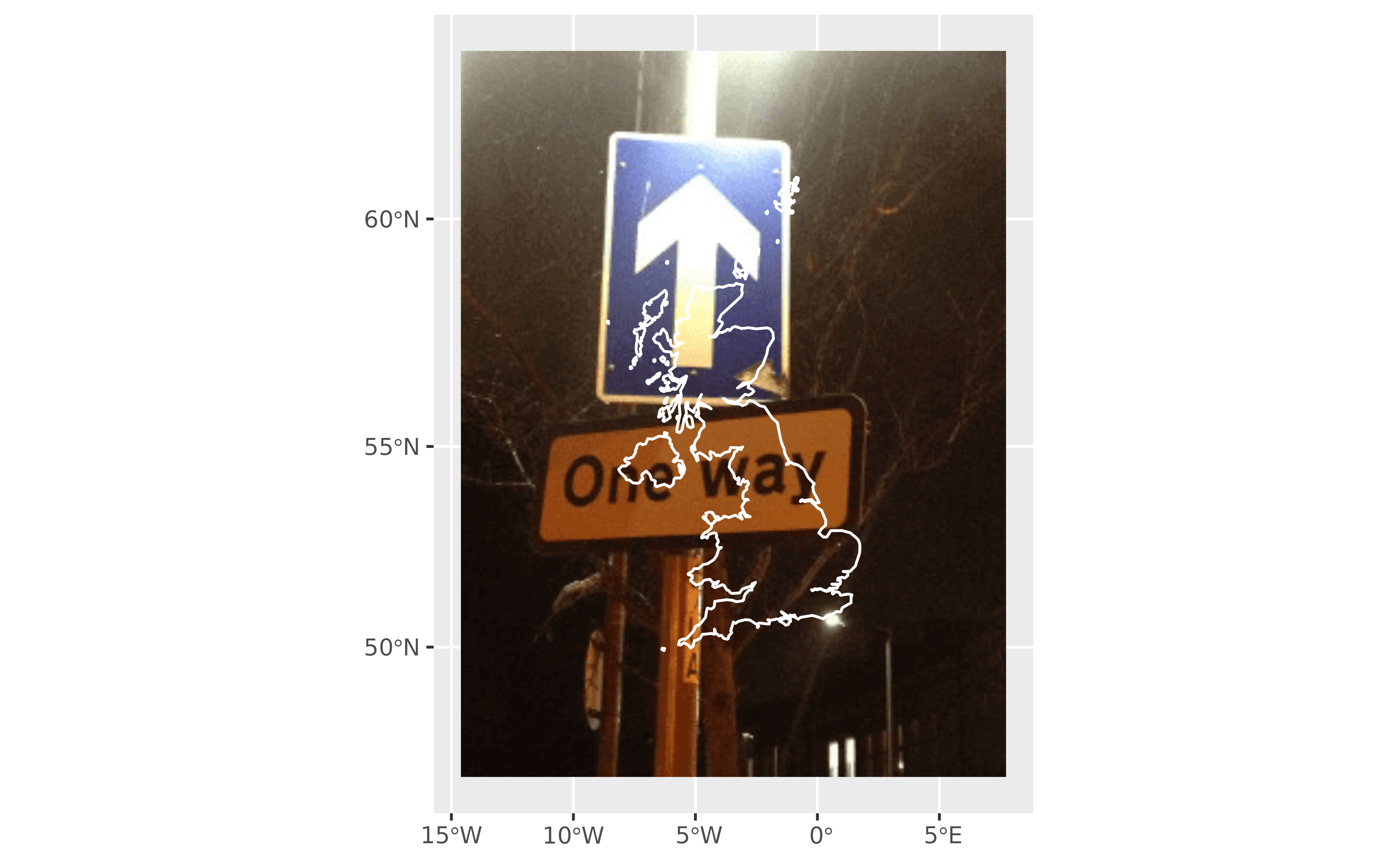
 # Expand the bounding box.
ex2 <- rasterpic_img(x, img, expand = 0.5)
autoplot(ex2) +
geom_sf(data = x, fill = NA, color = "white", linewidth = 0.5)
# Expand the bounding box.
ex2 <- rasterpic_img(x, img, expand = 0.5)
autoplot(ex2) +
geom_sf(data = x, fill = NA, color = "white", linewidth = 0.5)
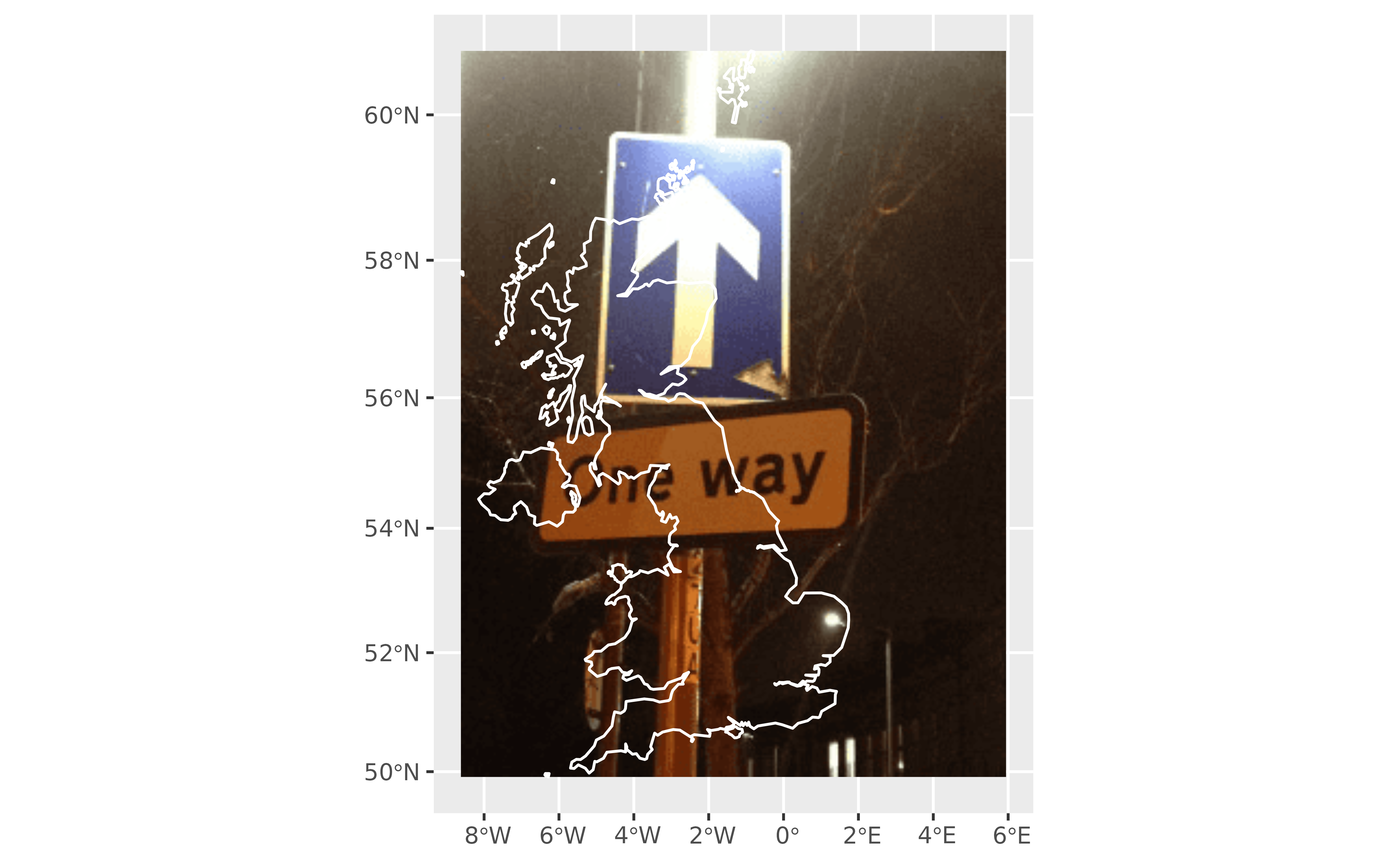
 # Align the image to the left edge.
ex3 <- rasterpic_img(x, img, halign = 0)
autoplot(ex3) +
geom_sf(data = x, fill = NA, color = "white", linewidth = 0.5) +
labs(title = "Align")
# Align the image to the left edge.
ex3 <- rasterpic_img(x, img, halign = 0)
autoplot(ex3) +
geom_sf(data = x, fill = NA, color = "white", linewidth = 0.5) +
labs(title = "Align")
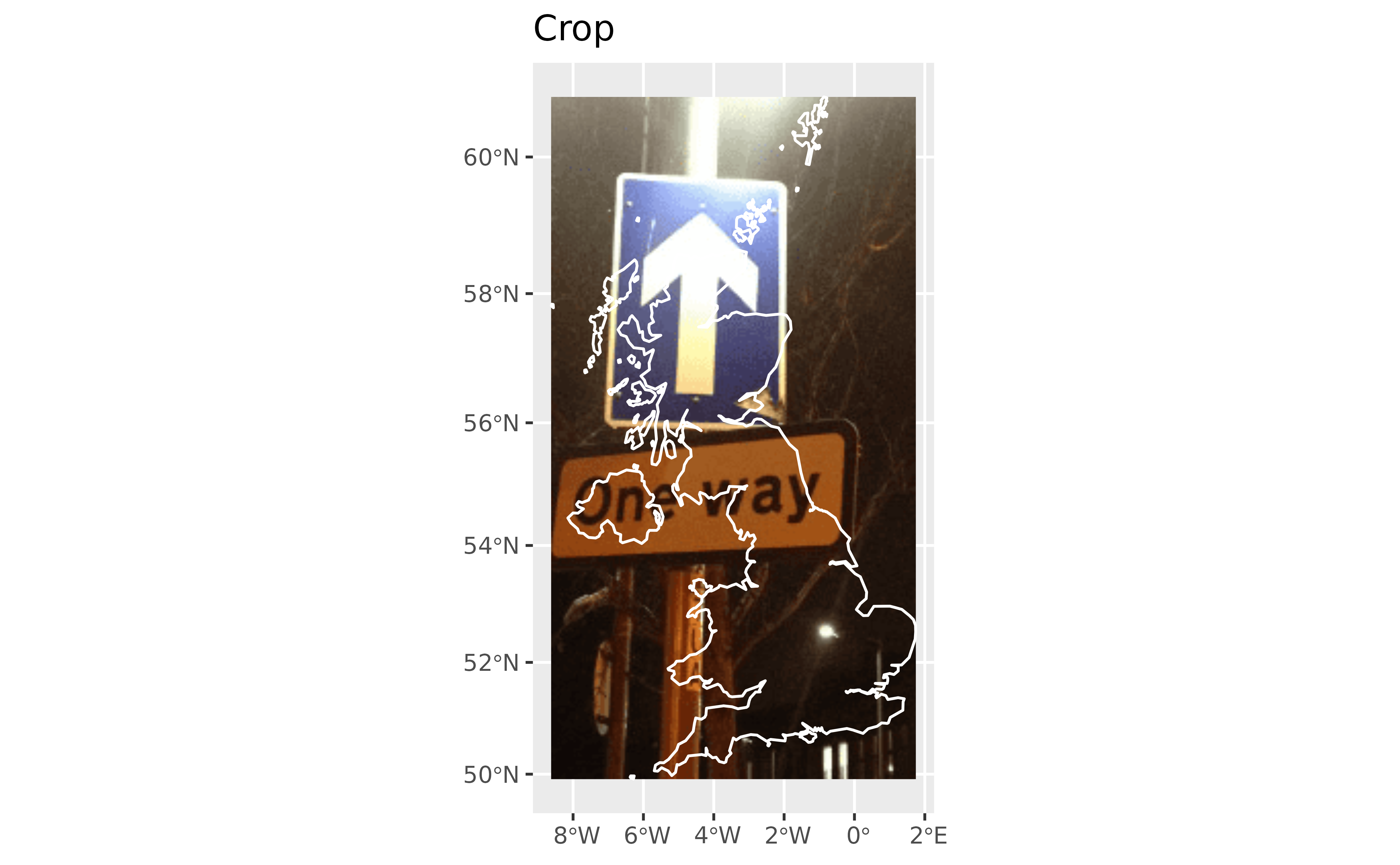
 # Crop to the bounding box.
ex4 <- rasterpic_img(x, img, crop = TRUE)
autoplot(ex4) +
geom_sf(data = x, fill = NA, color = "white", linewidth = 0.5) +
labs(title = "Crop")
# Crop to the bounding box.
ex4 <- rasterpic_img(x, img, crop = TRUE)
autoplot(ex4) +
geom_sf(data = x, fill = NA, color = "white", linewidth = 0.5) +
labs(title = "Crop")
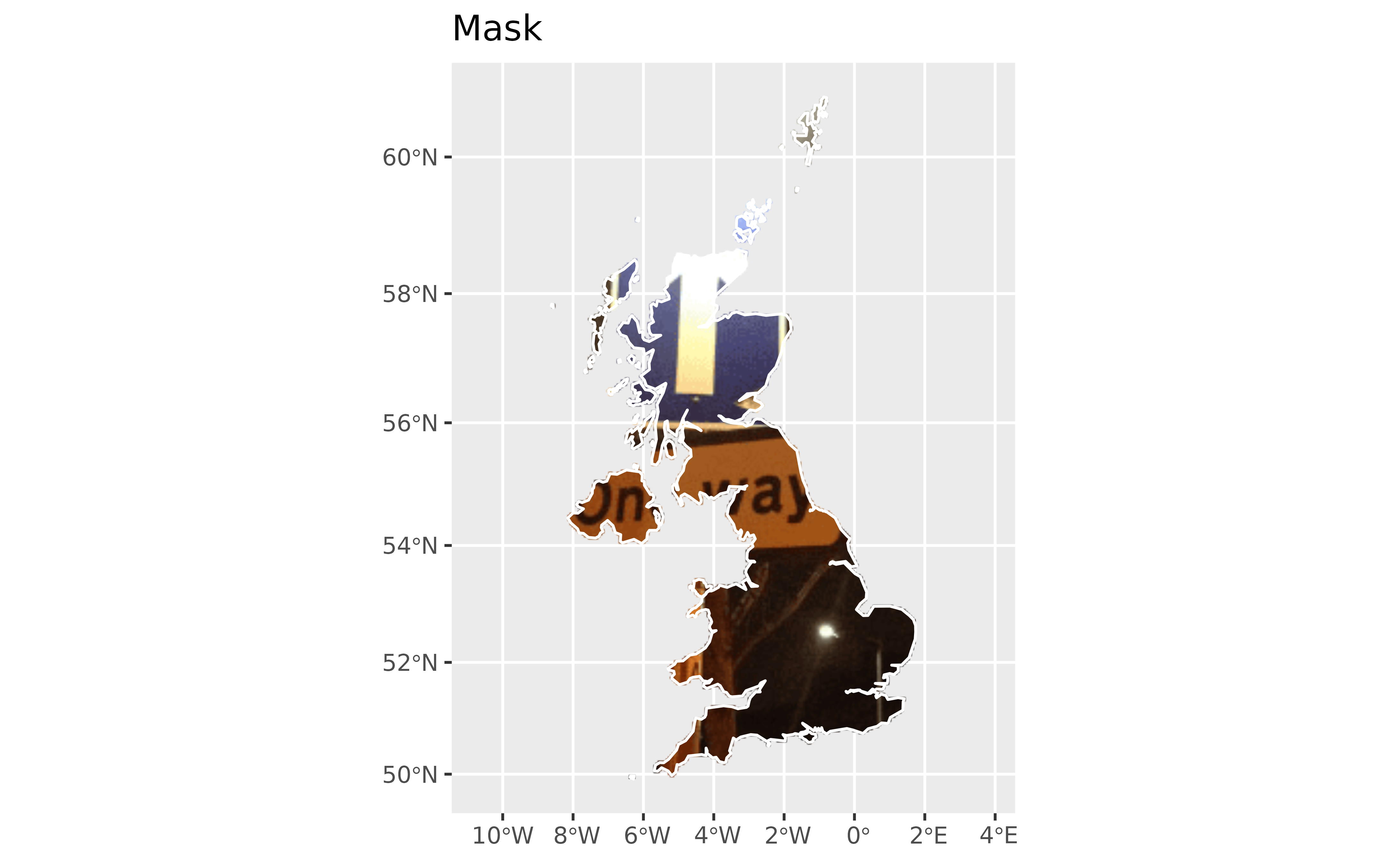
 # Mask to the vector shape.
ex5 <- rasterpic_img(x, img, mask = TRUE)
autoplot(ex5) +
geom_sf(data = x, fill = NA, color = "white", linewidth = 0.5) +
labs(title = "Mask")
# Mask to the vector shape.
ex5 <- rasterpic_img(x, img, mask = TRUE)
autoplot(ex5) +
geom_sf(data = x, fill = NA, color = "white", linewidth = 0.5) +
labs(title = "Mask")
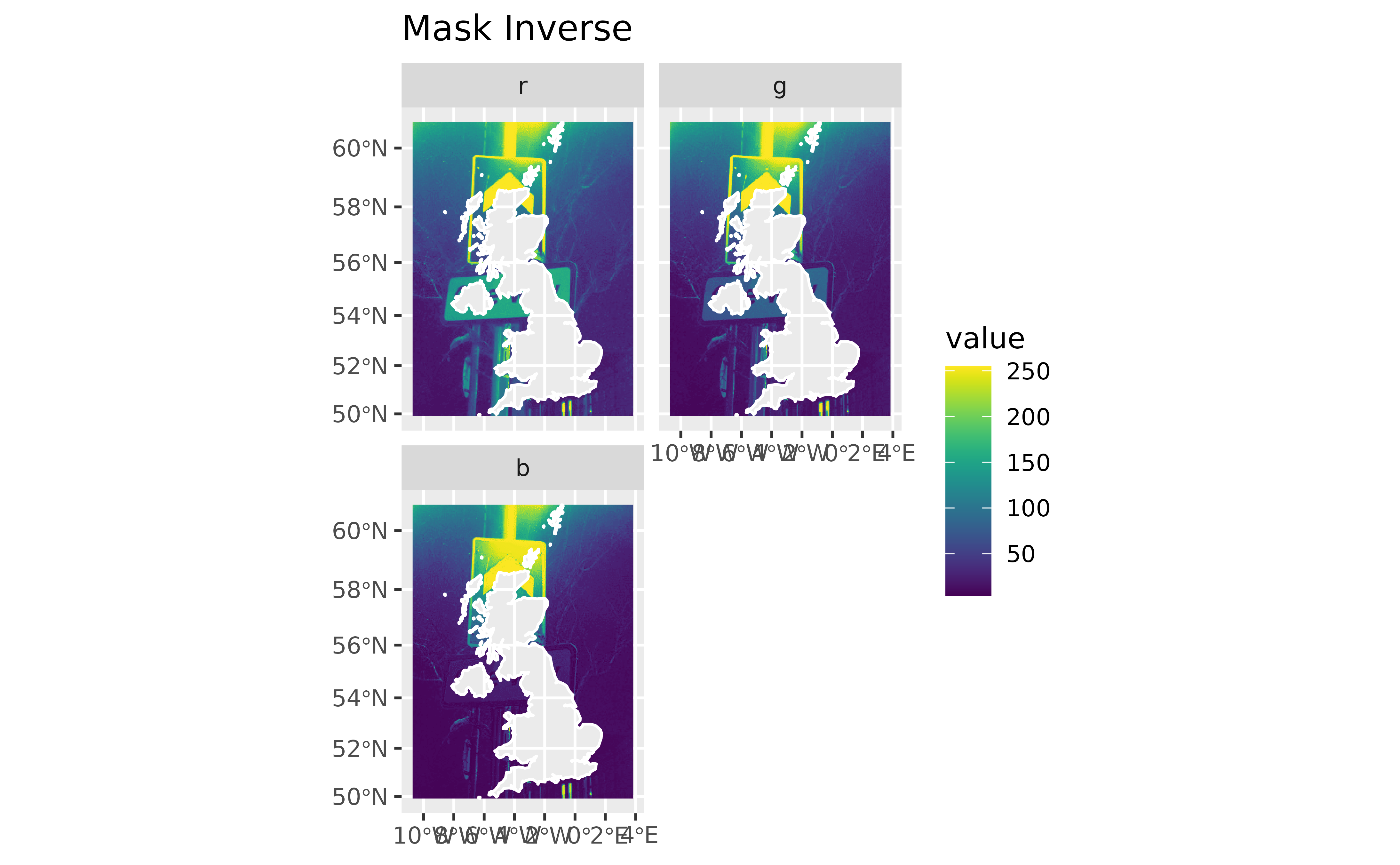
 # Mask outside the vector shape.
ex6 <- rasterpic_img(x, img, mask = TRUE, inverse = TRUE)
autoplot(ex6) +
geom_sf(data = x, fill = NA, color = "white", linewidth = 0.5) +
labs(title = "Mask Inverse")
# Mask outside the vector shape.
ex6 <- rasterpic_img(x, img, mask = TRUE, inverse = TRUE)
autoplot(ex6) +
geom_sf(data = x, fill = NA, color = "white", linewidth = 0.5) +
labs(title = "Mask Inverse")
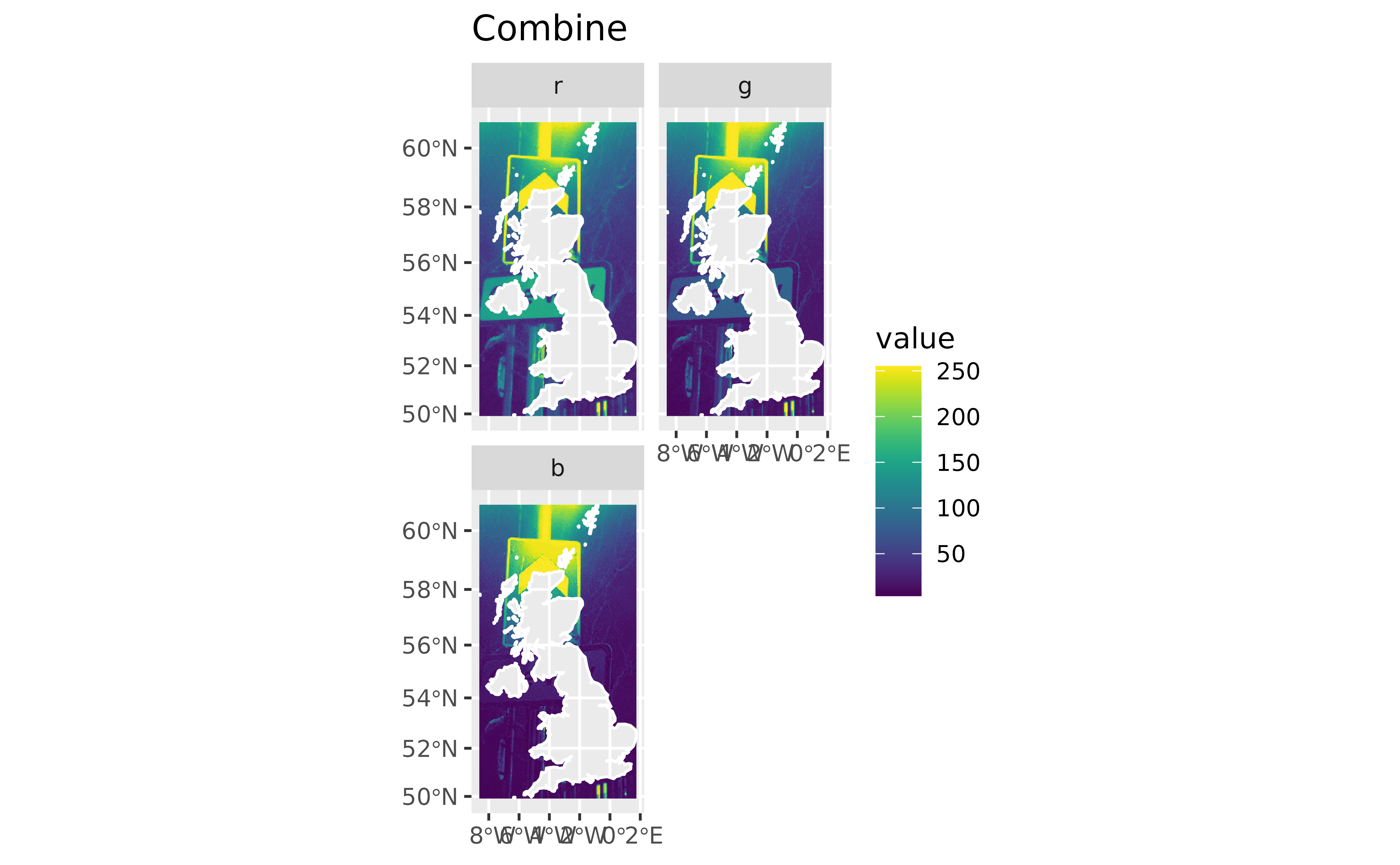
 # Combine cropping and inverse masking.
ex7 <- rasterpic_img(x, img, crop = TRUE, mask = TRUE, inverse = TRUE)
autoplot(ex7) +
geom_sf(data = x, fill = NA, color = "white", linewidth = 0.5) +
labs(title = "Combine")
# Combine cropping and inverse masking.
ex7 <- rasterpic_img(x, img, crop = TRUE, mask = TRUE, inverse = TRUE)
autoplot(ex7) +
geom_sf(data = x, fill = NA, color = "white", linewidth = 0.5) +
labs(title = "Combine")
 # }
# }