The package code is MIT licensed. Downloaded boundaries and figures derived from them retain the licenses and attribution requirements of geoBoundaries and their original sources. Check the boundary metadata before reuse.
Introduction
The geobounds package provides an interface for downloading and working with administrative boundaries from the geoBoundaries Global Database of Political Administrative Boundaries (Runfola et al. 2020).
The default gbOpen release type covers countries worldwide across multiple ADM levels. Its boundaries use multiple open licenses, including ODbL, CC BY and CC BY-SA. The package also supports gbHumanitarian and gbAuthoritative, which differ in their sources, validation processes and licensing. With geobounds, you can download boundaries as sf objects, inspect boundary metadata, cache downloaded files and integrate boundaries into spatial workflows.
This vignette keeps the main workflow in one place. It first explains how to choose the right boundary type, then covers cache management and finishes with a spatial analysis example.
Understanding the boundaries
The geoBoundaries database is designed for scientific and academic use, with quality assurance that includes manual review and hand digitization of physical maps where necessary.
This precision comes at a cost: some files can be quite large and may take longer to download. For visualization or general mapping purposes, we recommend using simplified boundaries by setting simplified = TRUE.
library(geobounds)
library(ggplot2)
library(dplyr)

# Compare resolutions.
norway <- gb_get_adm0("NOR") |>
  mutate(res = "Full resolution")
print(object.size(norway), units = "Mb")
#> 26.5 Mb

norway_simp <- gb_get_adm0(country = "NOR", simplified = TRUE) |>
  mutate(res = "Simplified")
print(object.size(norway_simp), units = "Mb")
#> 1.5 Mb

norway_all <- bind_rows(norway, norway_simp)

# Plot with ggplot2.
ggplot(norway_all) +
  geom_sf(fill = "#BA0C2F", color = "#00205B") +
  facet_wrap(vars(res)) +
  theme_minimal() +
  labs(
    caption = paste(
      "Sources: geoBoundaries and the original boundary provider,",
      "check gb_get_metadata() for the license"
    )
  )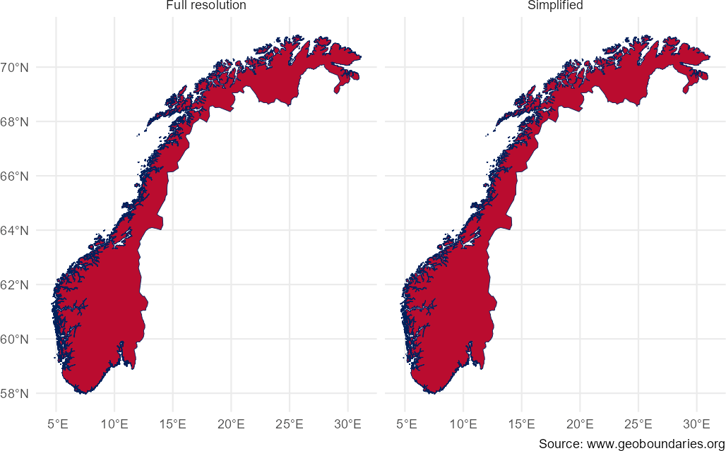
Comparison between full-resolution and simplified boundaries.
Individual country boundaries
The geoBoundaries API provides individual country boundaries that reflect how countries represent their own boundaries, without special identification of disputed areas.
Download individual country boundaries with gb_get() or the gb_get_adm*() wrappers. Borders are not guaranteed to align perfectly, gaps may exist between countries and disputed territories may not be represented consistently.
india_pak <- gb_get_adm0(c("India", "Pakistan"))

# Highlight the disputed Kashmir area.
ggplot(india_pak) +
  geom_sf(aes(fill = shapeName), alpha = 0.5) +
  scale_fill_manual(values = c("#FF671F", "#00401A")) +
  labs(
    fill = "Country",
    title = "Map of India and Pakistan",
    subtitle = "Note the overlap in the Kashmir region",
    caption = paste(
      "Sources: geoBoundaries and the original boundary providers,",
      "check gb_get_metadata() for licenses"
    )
  )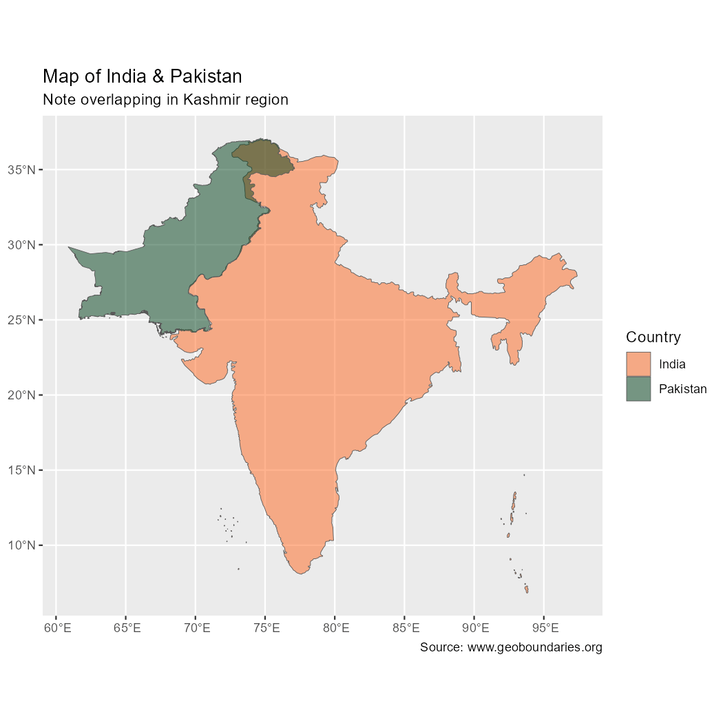
Map showing overlap in the disputed Kashmir area.
Each individual country boundary is governed by the license identified in its boundary metadata.
gb_get_metadata(c("India", "Pakistan"), adm_lvl = "ADM0") |>
  select(
    boundaryName,
    boundaryLicense,
    boundarySource,
    licenseSource
  )
#> # A tibble: 2 × 4
#>   boundaryName boundaryLicense                      boundarySource licenseSource
#>   <chr>        <chr>                                <chr>          <chr>
#> 1 India        CC0 1.0 Universal (CC0 1.0) Public … geoBoundaries… commons.wiki…
#> 2 Pakistan     Open Data Commons Open Database Lic… OpenStreetMap… www.openstre…
When sharing a boundary or a derived product, attribute geoBoundaries and the original providers shown in the metadata. Include the applicable license, link to its terms and indicate modifications when required. ODbL and CC BY-SA data may impose share-alike obligations beyond attribution.
Global composite boundaries
Use gb_get_world() for global composite boundaries that standardize disputed areas and fill gaps between borders. These boundaries are also known as Comprehensive Global Administrative Zones (CGAZ). They differ from individual country boundaries in three important ways:
- Extensive simplification keeps file sizes small enough for most desktop software.
- Disputed areas are removed and replaced with polygons following the definitions used by the CGAZ product.
- Gaps between borders are filled.
CGAZ boundaries and figures are not covered by the package’s MIT license. Follow the citation and use information included in each downloaded CGAZ archive.
cgaz_india_pak <- gb_get_world(c("India", "Pakistan"))

ggplot(cgaz_india_pak) +
  geom_sf(aes(fill = shapeName), alpha = 0.5) +
  scale_fill_manual(values = c("#FF671F", "#00401A")) +
  labs(
    fill = "Country",
    title = "Map of India and Pakistan",
    subtitle = "CGAZ does not overlap",
    caption = "Source: geoBoundaries (CGAZ)"
  )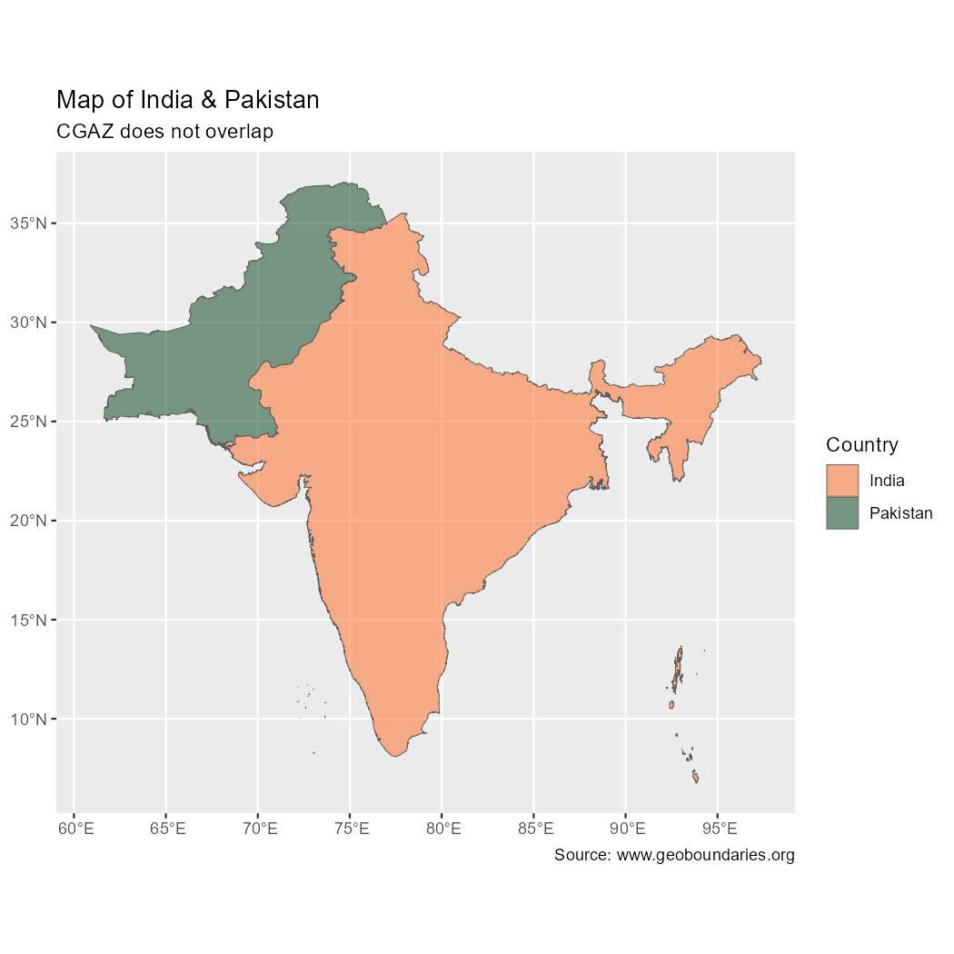
Map showing no overlap in Kashmir, provided by CGAZ.
Cache management and performance
geobounds stores downloaded files in a cache directory so repeated requests for the same country and ADM level can reuse the cached file. For example:
# Show the current cache directory.
current <- gb_detect_cache_dir()
#> ℹ 'C:\Users\RUNNER~1\AppData\Local\Temp\Rtmp6LfQDv'

current
#> [1] "C:\\Users\\RUNNER~1\\AppData\\Local\\Temp\\Rtmp6LfQDv"

# Change to a new cache directory.
newdir <- file.path(tempdir(), "geoboundvignette")
gb_set_cache_dir(newdir)
#> ✔ geobounds cache directory is 'C:\Users\RUNNER~1\AppData\Local\Temp\Rtmp6LfQDv/geoboundvignette'.
#> ℹ To use this cache directory in future sessions, call `gb_set_cache_dir()` with `install = TRUE`.

# Download the example data.
example <- gb_get_adm0("Vatican City", quiet = FALSE)
#> ℹ Downloading file from <https://github.com/wmgeolab/geoBoundaries/raw/9469f09/releaseData/gbOpen/VAT/ADM0/geoBoundaries-VAT-ADM0-all.zip>.
#> → Cache directory is 'C:\Users\RUNNER~1\AppData\Local\Temp\Rtmp6LfQDv/geoboundvignette/gbOpen'.

# Restore the cache directory.
gb_set_cache_dir(current)
#> ✔ geobounds cache directory is 'C:\Users\RUNNER~1\AppData\Local\Temp\Rtmp6LfQDv'.
#> ℹ To use this cache directory in future sessions, call `gb_set_cache_dir()` with `install = TRUE`.

current == gb_detect_cache_dir()
#> ℹ 'C:\Users\RUNNER~1\AppData\Local\Temp\Rtmp6LfQDv'
#> [1] TRUE
To clear the cache, use gb_clear_cache().
Use the cache_dir argument to set a cache directory for an individual function call.
Spatial analysis workflows
Because boundaries are returned as sf objects, you can combine them with other spatial data:
- Clip raster data to administrative units.
- Compute zonal statistics.
- Create choropleth maps.
- Perform spatial joins with survey or tabular data.
This example creates a choropleth map using metadata from individual country boundaries and global composite boundaries from CGAZ:
# Get boundary metadata.
latam_meta <- gb_get_metadata(adm_lvl = "ADM0") |>
  select(boundaryISO, boundaryName, Continent, worldBankIncomeGroup) |>
  filter(Continent == "Latin America and the Caribbean") |>
  glimpse()
#> Rows: 47
#> Columns: 4
#> $ boundaryISO          <chr> "ABW", "AIA", "ARG", "ATG", "BES", "BHS", "BLM", …
#> $ boundaryName         <chr> "Aruba", "Anguilla", "Argentina", "Antigua and Ba…
#> $ Continent            <chr> "Latin America and the Caribbean", "Latin America…
#> $ worldBankIncomeGroup <chr> "High-income Countries", "No income group availab…

# Adjust factors.
latam_meta$income_factor <- factor(
  latam_meta$worldBankIncomeGroup,
  levels = c(
    "High-income Countries",
    "Upper-middle-income Countries",
    "Lower-middle-income Countries",
    "Low-income Countries"
  )
)

# Get global composite boundaries from CGAZ.
latam_sf <- gb_get_world(adm_lvl = "ADM0") |>
  inner_join(latam_meta, by = c("shapeGroup" = "boundaryISO"))

ggplot(latam_sf) +
  geom_sf(aes(fill = income_factor)) +
  scale_fill_brewer(palette = "Greens", direction = -1) +
  guides(fill = guide_legend(position = "bottom", nrow = 2)) +
  coord_sf(
    crs = "+proj=laea +lon_0=-75 +lat_0=-15"
  ) +
  labs(
    title = "World Bank Income Group",
    subtitle = "Latin America and the Caribbean",
    fill = "",
    caption = "Source: geoBoundaries (CGAZ and gbOpen metadata)"
  )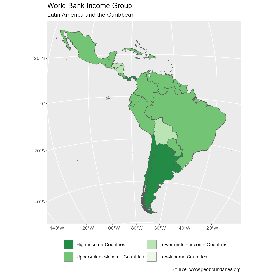
World Bank Income Group: Latin America and the Caribbean.
Summary
The geobounds package supports reproducible workflows for downloading, caching and visualizing administrative boundaries. The returned sf objects can be used directly in mapping, spatial analysis and data integration workflows.