
tidyterra
tidyterra provides methods from tidyverse packages for SpatRaster and SpatVector objects created with terra. It also provides geom_spat*() geoms and scales for plotting those objects with ggplot2.
Why tidyterra?
Spat* objects differ from regular data frames: they are S4 objects with their own syntax and computational methods (implemented in terra). By providing tidyverse verbs, especially dplyr and tidyr methods, tidyterra lets users manipulate Spat* objects in a style familiar from tabular data workflows.
terra is generally faster. Learning some terra syntax is recommended because tidyterra functions call the corresponding terra equivalents when possible.
A note for advanced terra users
tidyterra is not optimized for performance. Operations such as filter() and mutate() can be slower than their terra counterparts.
As a rule of thumb, tidyterra is most suitable for objects with fewer than 10,000,000 data slots, for example terra::ncell(a_rast) * terra::nlyr(a_rast) < 1e7.
Get started with tidyterra
Load tidyterra together with core tidyverse packages:
library(tidyterra)
#>
#> Attaching package: 'tidyterra'
#> The following object is masked from 'package:stats':
#>
#>     filter
library(dplyr)
#>
#> Attaching package: 'dplyr'
#> The following objects are masked from 'package:stats':
#>
#>     filter, lag
#> The following objects are masked from 'package:base':
#>
#>     intersect, setdiff, setequal, union
library(tidyr)
The following methods are available:
The following sections show some of these methods in action.
SpatRaster objects
This example uses a SpatRaster:
library(terra)
f <- system.file("extdata/cyl_temp.tif", package = "tidyterra")

temp <- rast(f)

temp
#> class       : SpatRaster
#> size        : 87, 118, 3  (nrow, ncol, nlyr)
#> resolution  : 3881.255, 3881.255  (x, y)
#> extent      : -612335.4, -154347.3, 4283018, 4620687  (xmin, xmax, ymin, ymax)
#> coord. ref. : World_Robinson (ESRI:54030)
#> source      : cyl_temp.tif
#> names       :   tavg_04,   tavg_05,   tavg_06
#> min values  :  1.885463,  5.817587, 10.463377
#> max values  : 13.283829, 16.740898, 21.113781

mod <- temp |>
  select(-1) |>
  mutate(newcol = tavg_06 - tavg_05) |>
  relocate(newcol, .before = 1) |>
  replace_na(list(newcol = 3)) |>
  rename(difference = newcol)

mod
#> class       : SpatRaster
#> size        : 87, 118, 3  (nrow, ncol, nlyr)
#> resolution  : 3881.255, 3881.255  (x, y)
#> extent      : -612335.4, -154347.3, 4283018, 4620687  (xmin, xmax, ymin, ymax)
#> coord. ref. : World_Robinson (ESRI:54030)
#> source(s)   : memory
#> names       : difference,   tavg_05,   tavg_06
#> min values  :   2.817647,  5.817587, 10.463377
#> max values  :   5.307511, 16.740898, 21.113781
In this example, we:
- Removed the first layer (
tavg_04). - Created a new layer
newcolas the difference betweentavg_06andtavg_05. - Relocated
newcolto be the first layer. - Replaced
NAvalues innewcolwith3. - Renamed
newcoltodifference.
Throughout these steps, core properties of the SpatRaster, including the number of cells, rows, columns, extent, resolution and CRS, remain unchanged. Other verbs such as filter(), slice() or drop_na() may alter these properties in a manner analogous to row operations on data frames.
SpatVector objects
Most dplyr and tidyr verbs work with SpatVector objects, so you can arrange, group and summarize their attributes.
lux <- system.file("ex/lux.shp", package = "terra")

v_lux <- vect(lux)

v_lux |>
  # Create categories.
  mutate(gr = cut(POP / 1000, 5)) |>
  group_by(gr) |>
  # Summarize by group.
  summarise(
    n = n(),
    tot_pop = sum(POP),
    mean_area = mean(AREA)
  ) |>
  # Arrange groups.
  arrange(desc(gr))
#> class       : SpatVector
#> geometry    : polygons
#> dimensions  : 3, 4  (geometries, attributes)
#> extent      : 5.74414, 6.528252, 49.44781, 50.18162  (xmin, xmax, ymin, ymax)
#> coord. ref. : lon/lat WGS 84 (EPSG:4326)
#> names       :          gr     n tot_pop mean_area
#> type        :      <fact> <int>   <num>     <num>
#> values      :   (147,183]     2  359427       244
#>               (40.7,76.1]     1   48187       185
#>               (4.99,40.7]     9  194391   209.778
The CRS is preserved during these operations. By default, summarise() merges geometries within each group.
Plotting with ggplot2
SpatRaster objects
When a SpatRaster has a CRS defined (terra::crs(a_rast) != ""), the geom uses ggplot2::coord_sf() and can reproject the raster to match other spatial layers.
library(ggplot2)

# Facet a SpatRaster object.

ggplot() +
  geom_spatraster(data = temp) +
  facet_wrap(~lyr) +
  scale_fill_whitebox_c(
    palette = "muted",
    na.value = "white"
  )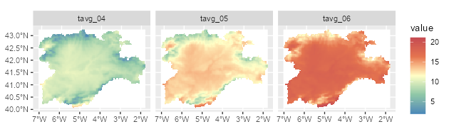
Faceted map using a SpatRaster object.
# Contour lines for a specific layer.

f_volcano <- system.file("extdata/volcano2.tif", package = "tidyterra")
volcano2 <- rast(f_volcano)

ggplot() +
  geom_spatraster(data = volcano2) +
  geom_spatraster_contour(data = volcano2, breaks = seq(80, 200, 5)) +
  scale_fill_whitebox_c() +
  coord_sf(expand = FALSE) +
  labs(fill = "elevation")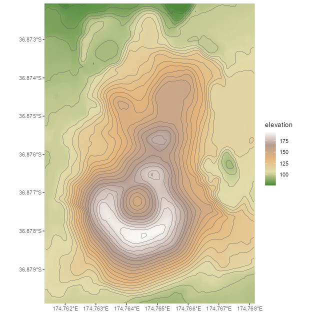
Contour line plot for a SpatRaster object.
# Filled contours.

ggplot() +
  geom_spatraster_contour_filled(data = volcano2) +
  scale_fill_whitebox_d(palette = "atlas") +
  labs(fill = "elevation")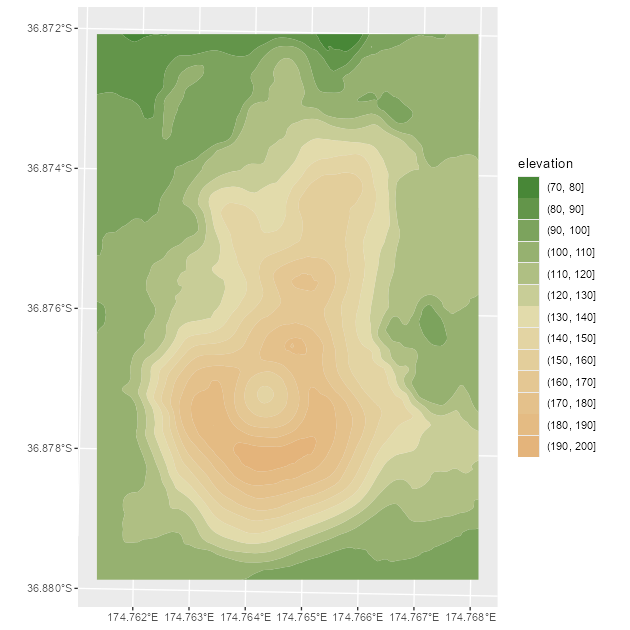
Filled contour plot for a SpatRaster object.
tidyterra also supports RGB SpatRaster objects for imagery:
# Read a vector.

f_v <- system.file("extdata/cyl.gpkg", package = "tidyterra")
v <- vect(f_v)

# Read a tile.
f_rgb <- system.file("extdata/cyl_tile.tif", package = "tidyterra")

r_rgb <- rast(f_rgb)

rgb_plot <- ggplot(v) +
  geom_spatraster_rgb(data = r_rgb) +
  geom_spatvector(fill = NA, size = 1)

rgb_plot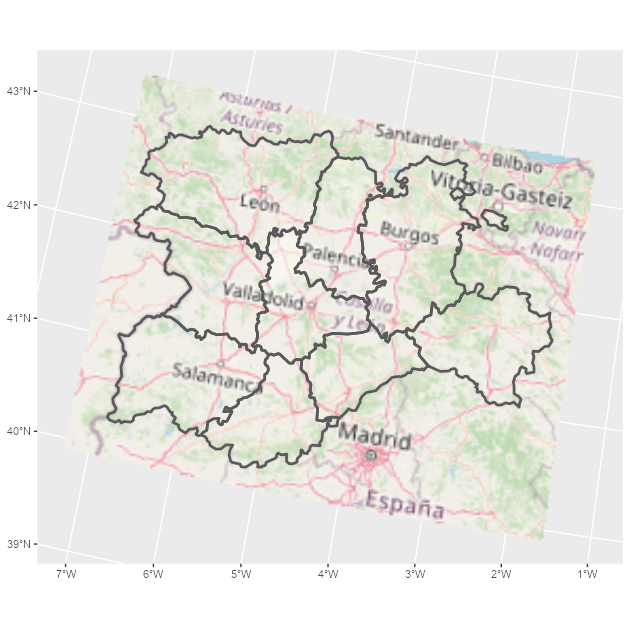
Map combining an RGB SpatRaster object and a SpatVector object.
tidyterra includes color scales and hypsometric tints suitable for topographic and bathymetric maps:
asia <- rast(system.file("extdata/asia.tif", package = "tidyterra"))

asia
#> class       : SpatRaster
#> size        : 164, 306, 1  (nrow, ncol, nlyr)
#> resolution  : 31836.23, 31847.57  (x, y)
#> extent      : 7619120, 1.736101e+07, -1304745, 3918256  (xmin, xmax, ymin, ymax)
#> coord. ref. : WGS 84 / Pseudo-Mercator (EPSG:3857)
#> source      : asia.tif
#> name        : file44bc291153f2
#> min value   :     -9558.467773
#> max value   :      5801.927246

ggplot() +
  geom_spatraster(data = asia) +
  scale_fill_hypso_tint_c(
    palette = "gmt_globe",
    labels = scales::label_number(),
    # Further refinements
    breaks = c(-10000, -5000, 0, 2000, 5000, 8000),
    guide = guide_colorbar(reverse = TRUE)
  ) +
  labs(
    fill = "elevation (m)",
    title = "Hypsometric map of Asia"
  ) +
  theme(
    legend.position = "bottom",
    legend.title.position = "top",
    legend.key.width = rel(3),
    legend.ticks = element_line(colour = "black", linewidth = 0.3),
    legend.direction = "horizontal"
  )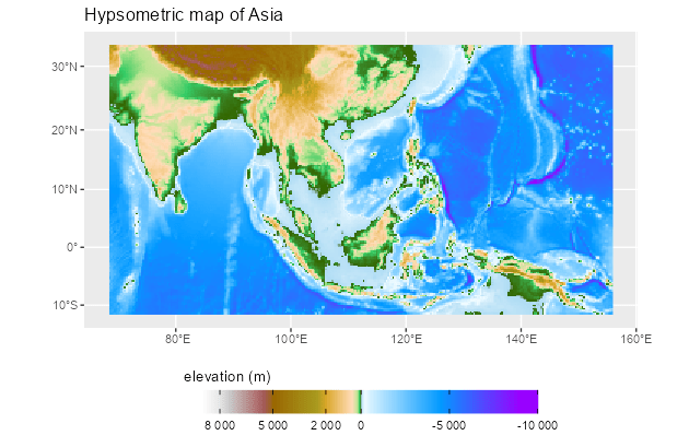
Map of Asia including hypsometric tints.
SpatVector objects
Plot SpatVector objects with geom_spatvector():
lux <- system.file("ex/lux.shp", package = "terra")

v_lux <- terra::vect(lux)

ggplot(v_lux) +
  geom_spatvector(aes(fill = POP), color = "white") +
  geom_spatvector_text(aes(label = NAME_2), color = "grey90") +
  scale_fill_binned(labels = scales::number_format()) +
  coord_sf(crs = 3857)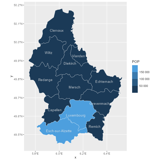
Choropleth map with a SpatVector object.
Internally, tidyterra converts SpatVector objects to sf objects with sf::st_as_sf() and then uses ggplot2::geom_sf() to render the layer.
You can also aggregate SpatVector objects:
# Dissolve by group.
v_lux |>
  # Create categories.
  mutate(gr = cut(POP / 1000, 5)) |>
  group_by(gr) |>
  # Summarize by group.
  summarise(
    n = n(),
    tot_pop = sum(POP),
    mean_area = mean(AREA)
  ) |>
  ggplot() +
  geom_spatvector(aes(fill = tot_pop), color = "black") +
  geom_spatvector_label(aes(label = gr)) +
  coord_sf(crs = 3857)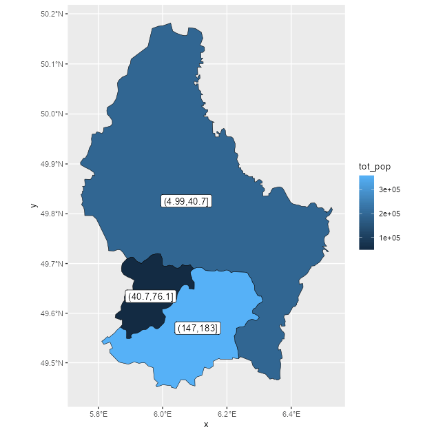
Dissolving SpatVector objects by group.
# Repeat while keeping internal boundaries.
v_lux |>
  # Create categories.
  mutate(gr = cut(POP / 1000, 5)) |>
  group_by(gr) |>
  # Summarize by group without dissolving.
  summarise(
    n = n(),
    tot_pop = sum(POP),
    mean_area = mean(AREA),
    .dissolve = FALSE
  ) |>
  ggplot() +
  geom_spatvector(aes(fill = tot_pop), color = "black") +
  geom_spatvector_label(aes(label = gr)) +
  coord_sf(crs = 3857)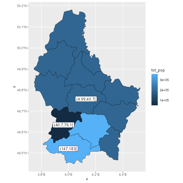
Aggregating SpatVector objects by group, keeping internal boundaries.