Group SpatVector objects by rows — rowwise.SpatVector • tidyterra

rowwise() allows you to compute on a SpatVector a row-at-a-time. This is most useful when a vectorised function doesn't exist.

Most dplyr verbs implementation in tidyterra preserve row-wise grouping. The exception is summarise.SpatVector(), which return a grouped SpatVector. You can explicitly ungroup with ungroup.SpatVector() or as_tibble(), or convert to a grouped SpatVector with group_by.SpatVector().

Usage

# S3 method for class 'SpatVector'
rowwise(data, ...)

Arguments

data

A SpatVector object. See Methods.

...

<tidy-select> Variables to be preserved when calling summarise.SpatVector(). This is typically a set of variables whose combination uniquely identify each row. See dplyr::rowwise().

NB: unlike group_by.SpatVector() you can not create new variables here but instead you can select multiple variables with (e.g.) everything().

Value

The same SpatVector object with an additional attribute.

Details

See Details on dplyr::rowwise().

Methods

Implementation of the generic dplyr::rowwise() function for SpatVector objects.

When mixing terra and dplyr syntax on a row-wise SpatVector (i.e, subsetting a SpatVector like v[1:3,1:2]) the groups attribute can be corrupted. tidyterra would try to re-generate the SpatVector. This would be triggered the next time you use a dplyr verb on your SpatVector.

Note also that some operations (as terra::spatSample()) would create a new SpatVector. In these cases, the result won't preserve the groups attribute. Use rowwise.SpatVector() to re-group.

Examples

library(terra)
library(dplyr)

v <- terra::vect(system.file("shape/nc.shp", package = "sf"))

# Select new births
nb <- v |>
  select(starts_with("NWBIR")) |>
  glimpse()
#> #  A SpatVector 100 x 2
#> #  Geometry type: Polygons
#> #  Geodetic CRS: lon/lat NAD27 (EPSG:4267)
#> #  Extent (x / y) : ([84° 19' 25.87" W / 75° 27' 25.12" W] , [33° 52' 55.17" N / 36° 35' 22.74" N])
#> 
#> $ NWBIR74 <dbl> 10, 10, 208, 123, 1066, 954, 115, 254, 748, 160, 550, 1243, 93…
#> $ NWBIR79 <dbl> 19, 12, 260, 145, 1197, 1237, 139, 371, 844, 176, 597, 1369, 1…

# Compute the mean of NWBIR on each geometry
nb |>
  rowwise() |>
  mutate(nb_mean = mean(c(NWBIR74, NWBIR79)))
#>  class       : SpatVector 
#>  geometry    : polygons 
#>  dimensions  : 100, 3  (geometries, attributes)
#>  extent      : -84.32385, -75.45698, 33.88199, 36.58965  (xmin, xmax, ymin, ymax)
#>  source      : nc.shp
#>  coord. ref. : lon/lat NAD27 (EPSG:4267) 
#>  names       : NWBIR74 NWBIR79 nb_mean
#>  type        :   <num>   <num>   <num>
#>  values      :      10      19    14.5
#>                     10      12      11
#>                    208     260     234

# Additional examples
# \donttest{
# use c_across() to more easily select many variables
nb |>
  rowwise() |>
  mutate(m = mean(c_across(NWBIR74:NWBIR79)))
#>  class       : SpatVector 
#>  geometry    : polygons 
#>  dimensions  : 100, 3  (geometries, attributes)
#>  extent      : -84.32385, -75.45698, 33.88199, 36.58965  (xmin, xmax, ymin, ymax)
#>  source      : nc.shp
#>  coord. ref. : lon/lat NAD27 (EPSG:4267) 
#>  names       : NWBIR74 NWBIR79     m
#>  type        :   <num>   <num> <num>
#>  values      :      10      19  14.5
#>                     10      12    11
#>                    208     260   234

# Compute the minimum of x and y in each row

nb |>
  rowwise() |>
  mutate(min = min(c_across(NWBIR74:NWBIR79)))
#>  class       : SpatVector 
#>  geometry    : polygons 
#>  dimensions  : 100, 3  (geometries, attributes)
#>  extent      : -84.32385, -75.45698, 33.88199, 36.58965  (xmin, xmax, ymin, ymax)
#>  source      : nc.shp
#>  coord. ref. : lon/lat NAD27 (EPSG:4267) 
#>  names       : NWBIR74 NWBIR79   min
#>  type        :   <num>   <num> <num>
#>  values      :      10      19    10
#>                     10      12    10
#>                    208     260   208

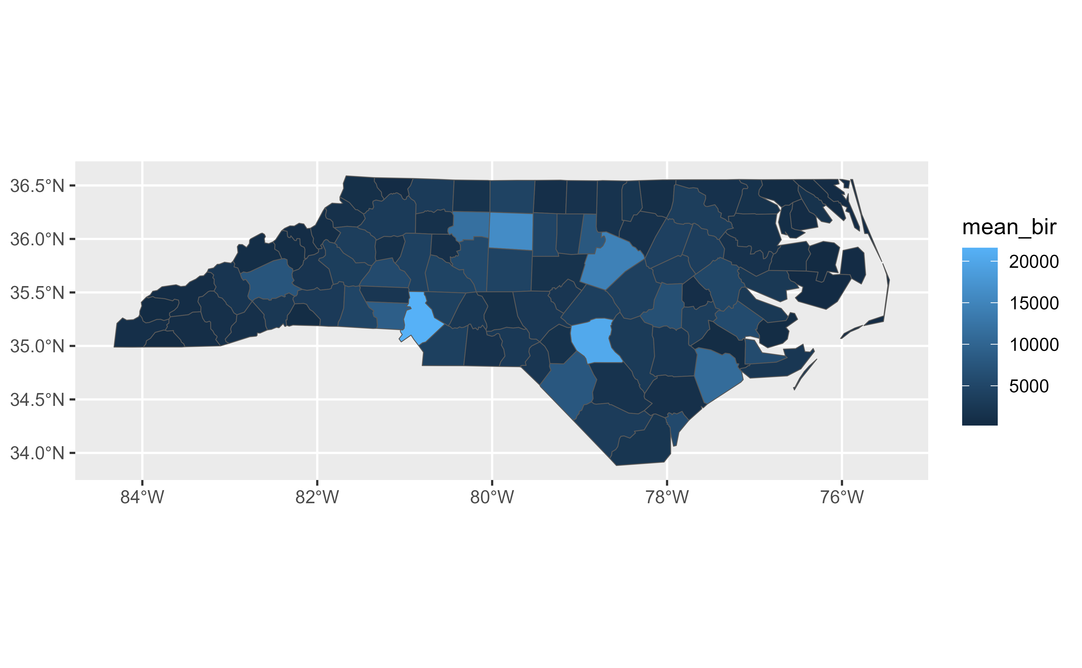
# Summarising
v |>
  rowwise() |>
  summarise(mean_bir = mean(BIR74, BIR79)) |>
  glimpse() |>
  autoplot(aes(fill = mean_bir))
#> #  A SpatVector 100 x 1
#> #  Geometry type: Polygons
#> #  Geodetic CRS: lon/lat NAD27 (EPSG:4267)
#> #  Extent (x / y) : ([84° 19' 25.87" W / 75° 27' 25.12" W] , [33° 52' 55.17" N / 36° 35' 22.74" N])
#> 
#> $ mean_bir <dbl> 1091, 487, 3188, 508, 1421, 1452, 286, 420, 968, 1612, 1035, …


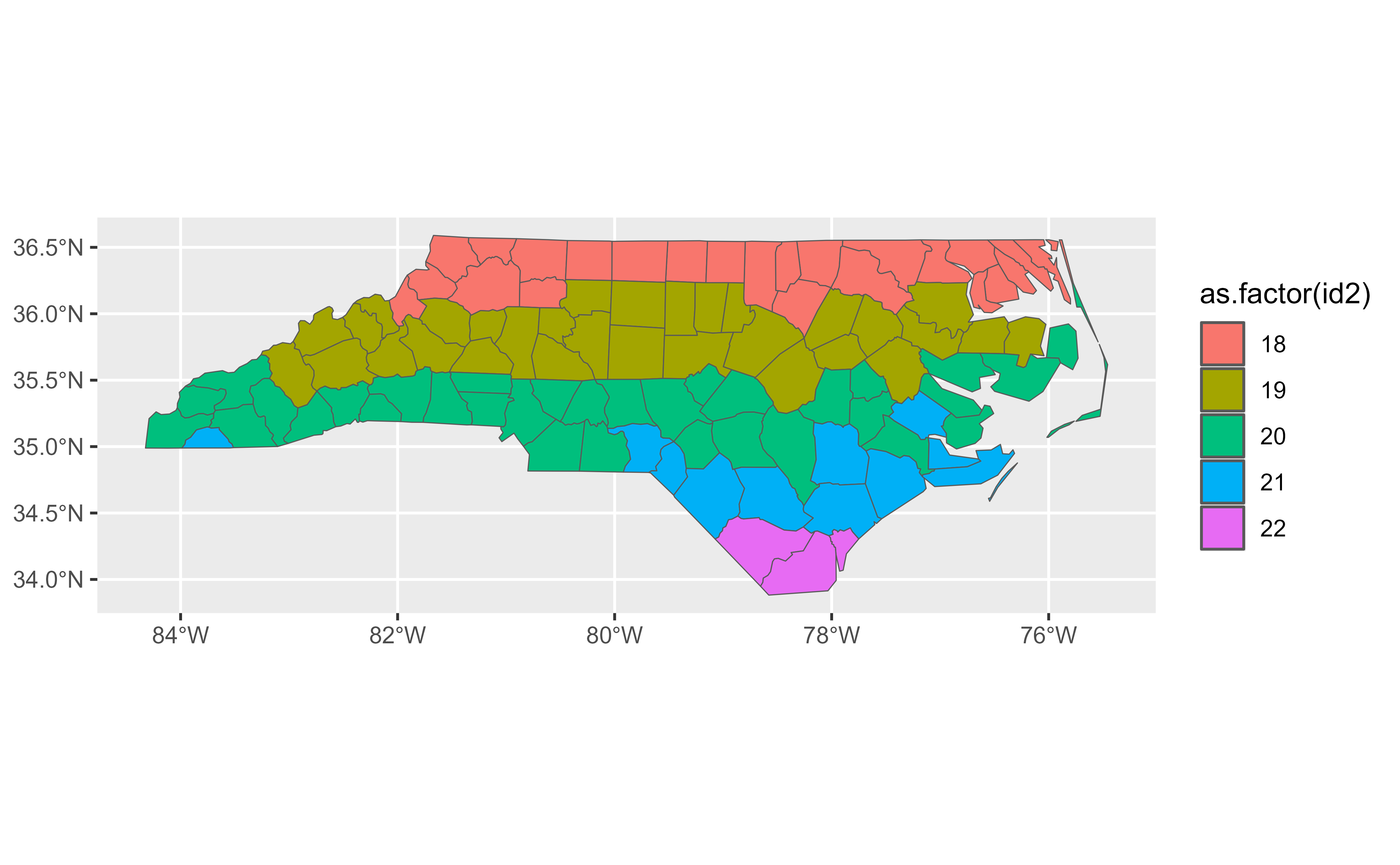
# Supply a variable to be kept
v |>
  mutate(id2 = as.integer(CNTY_ID / 100)) |>
  rowwise(id2) |>
  summarise(mean_bir = mean(BIR74, BIR79)) |>
  glimpse() |>
  autoplot(aes(fill = as.factor(id2)))
#> #  A SpatVector 100 x 2
#> #  Geometry type: Polygons
#> #  Geodetic CRS: lon/lat NAD27 (EPSG:4267)
#> #  Extent (x / y) : ([84° 19' 25.87" W / 75° 27' 25.12" W] , [33° 52' 55.17" N / 36° 35' 22.74" N])
#> 
#> Groups: id2 [2]
#> $ id2      <int> 18, 18, 18, 18, 18, 18, 18, 18, 18, 18, 18, 18, 18, 18, 18, 1…
#> $ mean_bir <dbl> 1091, 487, 3188, 508, 1421, 1452, 286, 420, 968, 1612, 1035, …

# }

Group `SpatVector` objects by rows